Introduction

This post develops a physics-informed neural network (PINN) for relativistic hydrodynamics (RHD), with the goal of using the differentiability of the network to compute derivatives of $T^{\mu\nu}$ with respect to transport coefficients and equation-of-state parameters directly via autograd. This recasts parameter inference as gradient-based optimization rather than posterior sampling over a Gaussian-process surrogate, the current standard in the heavy-ion community. Stage 1, presented here, is Bjorken flow in 1+1 dimensions, with and without viscosity.

Relativistic hydrodynamics is the workhorse description of the quark-gluon plasma (QGP) produced in heavy-ion collisions at RHIC and the LHC. The success of the hydrodynamic picture, that a system of $\mathcal{O}(10^3)$ particles evolving for $\mathcal{O}(10\,\text{fm}/c)$ can be described by a fluid with small but nonzero specific shear viscosity $\eta/s$, is one of the central results of the heavy-ion program. Extracting transport coefficients and the equation of state from experimental data requires running large numbers of hydrodynamic simulations across the parameter space, and the standard approach is to train Gaussian Process Emulators (GPEs) on a designed grid of simulations and perform Bayesian inference against measured observables.

Rather than emulate the parameter-to-observable map with a surrogate fit to discrete training points, the PINN represents the solution itself as a smooth, differentiable function of both spacetime coordinates and physical parameters. The same network that gives $T^{\mu\nu}(\tau, \eta\,;\,\eta/s, c_s^2, \ldots)$ also gives $\partial T^{\mu\nu} / \partial(\eta/s)$ at any point in the domain, for free.

PINNs differ from traditional solvers in how the solution is represented. A finite-difference or finite-volume scheme advances a discretized state forward in a chosen dynamical variable (here $t$),

where $\mathbf{U}^n$ is the discretized state at step $n$ and $\mathcal{L}$ encodes the spatial discretization of the equations of motion. The output is a grid of values that approximates the solution at successive timesteps.

A PINN instead represents the solution as a neural network $u_\theta(x,t)$ over the entire spacetime domain, with the weights $\theta$ trained to minimize a loss built from the equations of motion and the boundary conditions. There is no integration timestep; each training iteration is a refinement of the global representation. The derivatives that appear in the PDE residual are computed exactly via automatic differentiation, not approximated by finite differences.

This post is organized as follows. Section 2 states the equations of motion for RHD and the corresponding PINN loss. Section 3 presents Stage 1: Bjorken flow with and without viscosity, covering the inviscid case, the Navier-Stokes pathology, and the Israel-Stewart formulation including the hydrodynamic attractor. Section 4 turns to the inverse problem, first with a fixed equation of state and then with parametric and learned (neural) equations of state. Section 5 extends the program to 2+1 dimensions via Gubser flow. Mathematical details of the exact solutions are collected in the Appendix.

RHD PINN formulation

Equations of motion

Relativistic hydrodynamics is the conservation of the stress-energy tensor,

closed by an equation of state and, in the dissipative case, by relaxation equations for the viscous components. Decomposing $T^{\mu\nu}$ relative to the fluid four-velocity $u^\mu$ gives

where $\varepsilon$ is the energy density in the local rest frame, $p$ is the equilibrium pressure fixed by the EoS $p(\varepsilon)$, $\Delta^{\mu\nu} = g^{\mu\nu} + u^\mu u^\nu$ projects onto the spatial hypersurface orthogonal to $u^\mu$, and $\pi^{\mu\nu}$ and $\Pi$ are the shear and bulk viscous corrections.

In the ideal limit $\pi^{\mu\nu} = 0$ and $\Pi = 0$; in first-order (Navier-Stokes) hydrodynamics they are algebraic functions of the gradients of $u^\mu$; in second-order (Israel-Stewart) hydrodynamics they satisfy their own relaxation equations, which restore causality and stability lost in the first-order theory.

Stage 1 specializes these equations to Bjorken flow, where boost invariance and transverse homogeneity reduce the system to a single scalar ODE in proper time $\tau$; the reduction and the resulting relaxation equations for $\pi$ are developed there. Detailed derivations are collected in the Appendix.

PINN loss

The following states the loss for the Bjorken case developed in Stage 1; the form adapts straightforwardly to other geometries. The PINN represents the solution as a neural network $\varepsilon_\theta(\tau\,;\,\lambda)$ parameterized by weights $\theta$, where $\lambda$ collects any conditioning parameters (EoS, transport coefficients) that are exposed as inputs for the inverse-problem stages. The initial condition $\varepsilon_\theta(\tau_0\,;\,\lambda) = \varepsilon_0$ is built in by the ansatz

where $\delta_\theta$ is the neural network output. The ansatz exactly satisfies $\varepsilon_\theta(\tau_0) = \varepsilon_0$, removing one penalty from the loss, and exposes the ideal Bjorken scaling $\varepsilon \sim \tau^{-4/3}$ as the $\delta_\theta = 0$ solution, so the network learns only the deviation from the leading power law. A simpler additive ansatz $\varepsilon_\theta = \varepsilon_0 + (\tau - \tau_0)\,\mathrm{NN}_\theta$ also enforces the IC but hits a $\sim 4\%$ max-rel-err floor; the physics-aware form drops this to $\sim 2 \times 10^{-4}$.

The training objective is the squared PDE residual averaged over a set of collocation points ${\tau_i}$ in the domain,

with the time derivative computed by autograd through the network. For the Israel-Stewart case the loss extends to include the residual of the relaxation equation for $\pi$ and a second network output representing $\pi(\tau;\lambda)$.

When fitting to data (as in the inverse-problem stage), a supervised term is added,

where $\mathcal{L}_{\text{phys}}$ may be used to collect soft physical constraints (causality $c_s^2 \le 1$, thermodynamic stability $c_s^2 \ge 0$, and any limiting-case anchors such as a conformal high-temperature limit on the EoS). Collocation points are sampled log-uniformly in $\tau$, reflecting the scale-free character of the expansion, and resampled periodically during training. Optimization runs Adam followed by additional iterations with L-BFGS.

Stage 1: Bjorken flow

Bjorken’s model assumes boost-invariant longitudinal expansion and transverse homogeneity, the appropriate idealization for the mid-rapidity slice of a high-energy heavy-ion collision shortly after the two nuclei pass through each other. In Milne coordinates $(\tau, \eta, x, y)$, with $\tau = \sqrt{t^2 - z^2}$ and $\eta = \tfrac{1}{2}\log[(t+z)/(t-z)]$, boost invariance is the statement that all hydrodynamic fields depend only on $\tau$, and transverse homogeneity removes the $x, y$ dependence. The fluid four-velocity is at rest in the comoving frame, $u^\mu = (1, 0, 0, 0)$, and the only nontrivial equation is the scalar evolution equation derived above.

This drastic dimensional reduction is what makes Bjorken flow the canonical benchmark: every regime of relativistic hydrodynamics, ideal, first-order viscous, second-order relaxational, admits a closed-form or quadrature solution that the PINN can be compared against directly. Detailed derivations of the analytic results quoted here are collected in the Appendix.

I train Stage 1 in three regimes, each adding a piece of physics to the previous.

Ideal Bjorken flow

In the inviscid limit, with a conformal equation of state $p = c_s^2 \varepsilon$ and $c_s^2 = 1/3$, the energy equation integrates to the celebrated Bjorken cooling law,

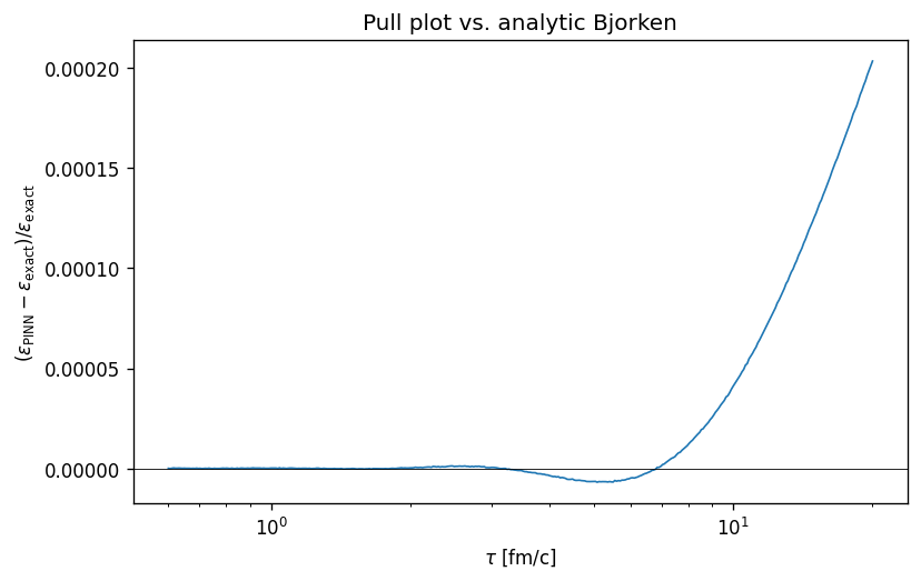
The exponent is set by the sound speed: a stiffer EoS cools faster, since the work done by pressure against the expansion is larger. This single power law is the cleanest possible target for the PINN. Training the conformal-EoS PINN against the residual of the scalar equation alone (no supervised data term) recovers the power-law solution with maximum relative error $2.07\times 10^{-4}$ across the domain $\tau \in [0.6, 20]\,\text{fm}/c$.

FIXME caption — pull plot $(\varepsilon_\theta - \varepsilon_{\text{exact}})/\varepsilon_{\text{exact}}$ vs $\tau$ for the ideal conformal-EoS run (conformal_smoke). Pulls are flat across the domain at the $10^{-4}$ level.

A finer test than pointwise accuracy is recovery of the exponent itself. Fitting $\log \varepsilon_\theta$ against $\log \tau$ on a held-out grid returns $1 + c_s^2$ to comparable precision, confirming that the PINN has learned the correct asymptotic scaling rather than memorizing a high-precision interpolant.

Navier-Stokes and its pathology

Adding shear viscosity in the first-order Navier-Stokes closure $\pi = (4\eta/3)/\tau$ introduces an entropy-producing correction. The energy equation becomes

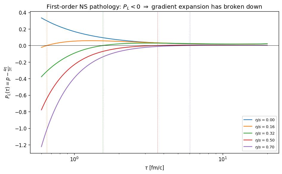
and the viscous term slows the cooling. At late times, when $\tau$ is large and $\pi/(\varepsilon+p) \ll 1$, this works well and matches the perturbative expansion in $\eta/s$ around the ideal solution. The pathology appears at early times. The effective longitudinal pressure $p_L = p - \pi$ can go negative when the algebraic NS expression for $\pi$ is large compared to the equilibrium pressure, signalling that the gradient expansion has broken down and that the first-order theory is no longer a controlled description. This is not a numerical artifact but a feature of the closure: NS hydrodynamics is acausal and linearly unstable around equilibrium, and Bjorken flow exposes the breakdown unambiguously because the relevant gradient ($1/\tau$) is large at early proper times.

FIXME caption — effective longitudinal pressure $p_L = p - \pi$ vs $\tau$ for several $\eta/s$ values. The shaded region $p_L < 0$ is the breakdown of first-order hydrodynamics. At $\eta/s = 0.32$ the minimum reaches $p_L = -0.378$ at $\tau = 0.6\,\text{fm}/c$.

The PINN reproduces this behavior faithfully. Training with the NS source recovers the analytic NS solution within the regime where it is well-defined, and the predicted $p_L$ crosses zero at the proper time predicted by the closed-form expression. The PINN does not “fix” the pathology, nor should it: the loss enforces the equation it is given.

Israel-Stewart and the hydrodynamic attractor

The second-order Israel-Stewart formulation promotes $\pi$ to an independent dynamical field with its own relaxation equation, restated here for convenience,

The relaxation time $\tau_\pi$ is the timescale on which $\pi$ relaxes toward its NS value. For $\tau \gg \tau_\pi$ the system tracks NS; at early times the relaxation regularizes the closure and the theory remains causal and stable.

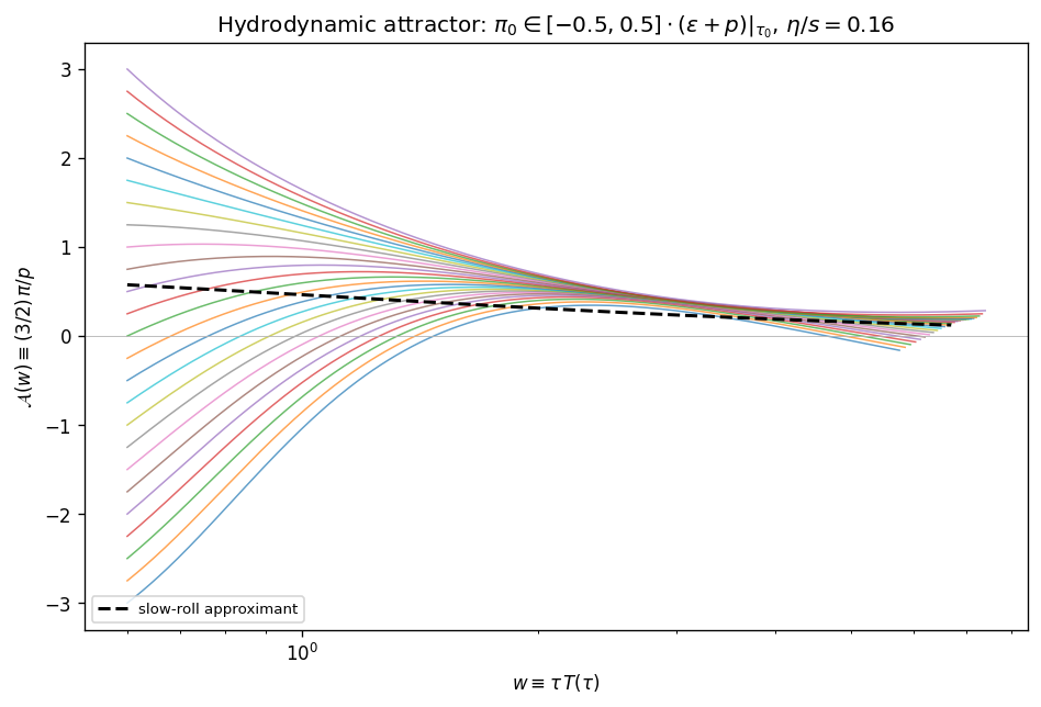
A central feature of the IS Bjorken system is the existence of a hydrodynamic attractor. Trajectories launched from a wide range of initial conditions for $\pi(\tau_0)$ collapse onto a single universal curve in the $(w, \pi/(\varepsilon+p))$ plane, where $w = \tau T$ is the dimensionless time variable that absorbs the natural scale. The attractor is approached on a timescale set by $\tau_\pi$, faster than the timescale on which the system becomes hydrodynamic in the gradient-expansion sense.

I train the IS PINN with the two-network architecture, one network for $\varepsilon_\theta(\tau)$ and a second for the normalized shear $\tilde\pi_\theta = \pi_\theta/(\varepsilon+p)$. The loss is the sum of the residuals of both equations, evaluated on the same log-spaced collocation grid. The smoke-test run reaches a total residual loss of $2.3\times 10^{-9}$ with a maximum normalized shear residual of $1.6\times 10^{-4}$, and the predicted effective longitudinal pressure stays positive everywhere in the domain, in contrast to NS.

For the attractor test, initial conditions $\pi(\tau_0)$ are swept while keeping $\eta/s$ fixed. Twenty-five trajectories with $\pi(\tau_0)$ spanning the physical range are propagated forward, and their normalized shear is plotted against the dimensionless time $w = \tau T$. The trajectories collapse onto the universal curve well before $w \sim 1$, with a contraction ratio (initial spread divided by spread at $w = 1$) of $21.5$.

FIXME caption — normalized shear $\tilde\pi = \pi/(\varepsilon + p)$ vs dimensionless time $w = \tau T$ for 25 initial conditions $\pi(\tau_0)$. Trajectories collapse onto the attractor before $w \sim 1$; contraction ratio $21.5$.

The PINN recovers the attractor without being told about it. The collapse of initial conditions is a property of the equations of motion, and the network learns it as a byproduct of minimizing the residual loss over the conditioning range.

Solution properties

Beyond pointwise accuracy, the trained IS model supports a battery of post-processing diagnostics that characterize the structure of the solution. Three are quoted here; full panels appear in the figure block below.

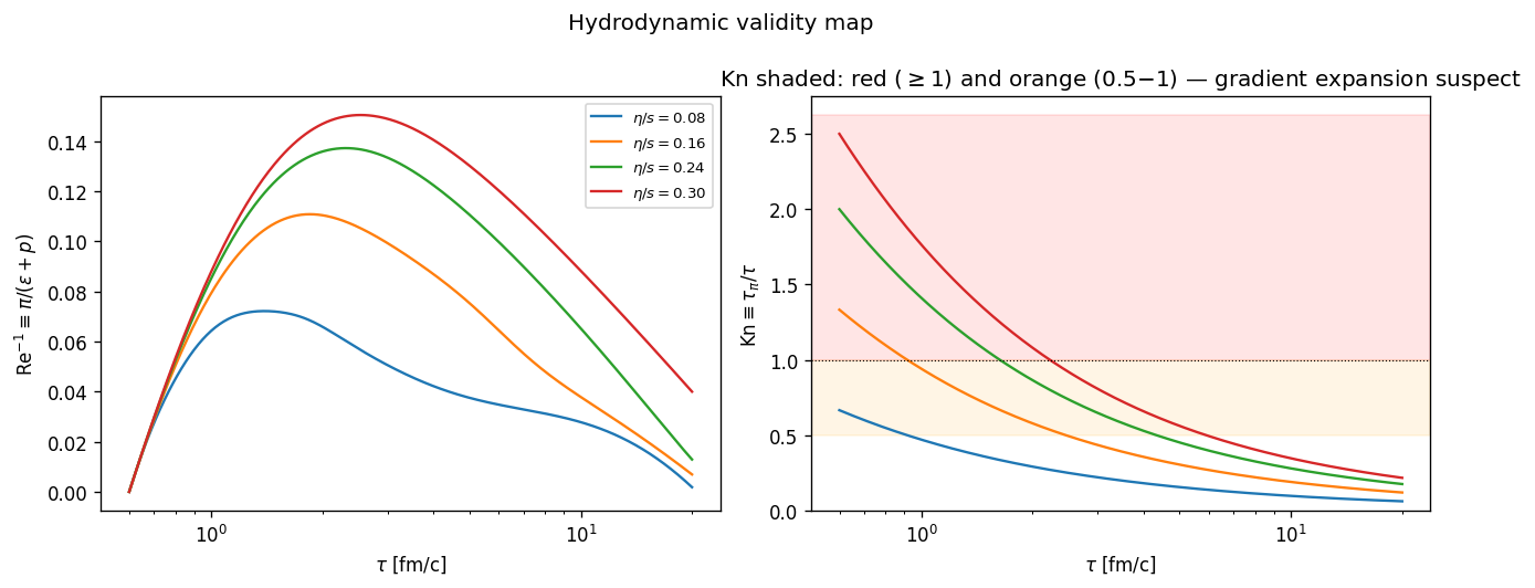
Knudsen map. The dimensionless Knudsen number $\mathrm{Kn} = \tau_\pi / \tau$ measures the local size of the gradient expansion’s small parameter. The locus $\mathrm{Kn} = 1$ marks the boundary between the hydrodynamic and pre-hydrodynamic regions of the $(\tau, \eta/s)$ plane. The trained PINN places this boundary at $\tau \approx {0.91, 1.62, 2.22}\,\text{fm}/c$ for $\eta/s = {0.16, 0.24, 0.30}$, consistent with the analytic estimate.

Sensitivity heatmap. The autograd derivative $\partial \varepsilon_\theta / \partial(\eta/s)$ is plotted across the $(\tau, \eta/s)$ plane. A finite-difference cross-check at a few sample points agrees with the autograd value to $2.9\times 10^{-4}$, validating that the gradient channel works at the level needed for downstream inference.

Forgetting time. The time $w^\star$ at which the spread across initial conditions for $\pi$ has decayed by a fixed factor quantifies memory of the initial state. Across the conditioning range, $w^\star$ has median $3.66$ and maximum $3.94$, well inside the hydrodynamic regime.

FIXME caption — Knudsen number $\mathrm{Kn} = \tau_\pi/\tau$ across $(\tau, \eta/s)$, with the $\mathrm{Kn} = 1$ contour separating hydrodynamic from pre-hydrodynamic regions.

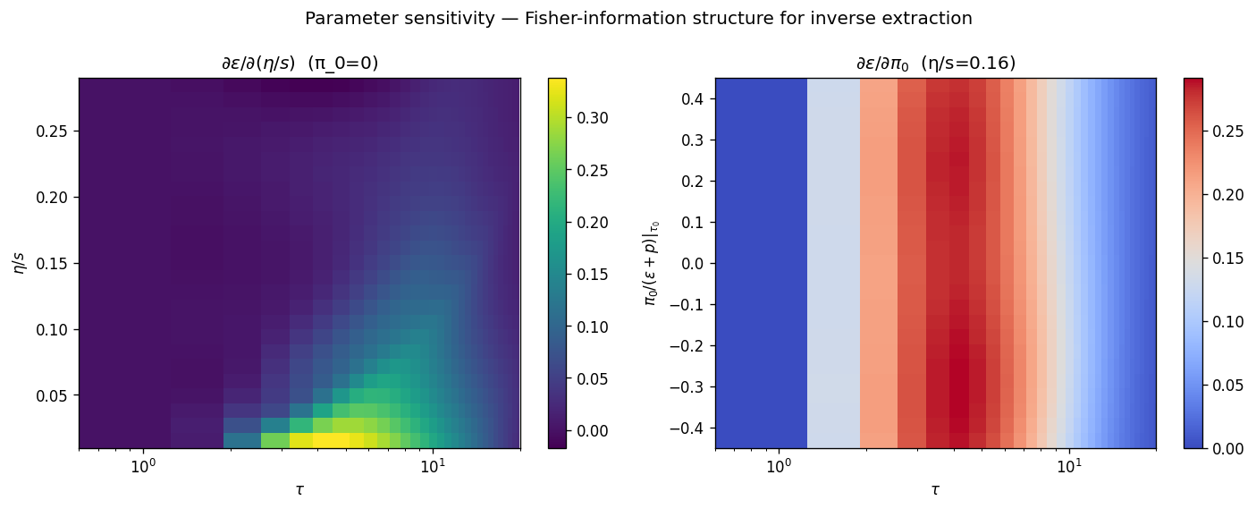FIXME caption — $\partial\varepsilon/\partial(\eta/s)$ from autograd across the $(\tau, \eta/s)$ plane.

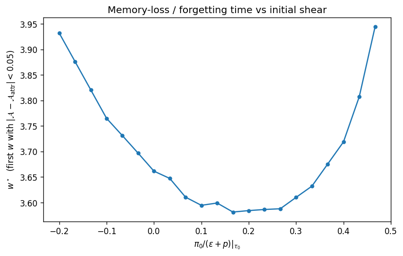FIXME caption — distribution of $w^\star$, the dimensionless time at which the spread across initial conditions for $\pi$ has decayed by a fixed factor.

Stage 1 summary

Across the three regimes the PINN reproduces the analytic structure of Bjorken hydrodynamics: the power-law cooling of the ideal case, the controlled validity domain of the NS closure, and the attractor behavior of IS. None of these features is hard-coded; each is learned from the residual of the equation it solves. This establishes the forward solver as a working component, which Stage 2 will use as the building block for differentiable inverse-problem inference.

Stage 2: Inverse Problem and Differentiability

Conditional PINN setup

Stub. Generalize from a single trained solution to a family of solutions parameterized by physical inputs $\lambda$ (EoS coefficients, transport coefficients). The network takes $(\log\tau, \lambda_{\text{norm}})$ as input, with $\lambda$ normalized to $[-1, 1]$, and the ansatz from the formulation section is unchanged. Loss is the PDE residual averaged jointly over collocation points in $\tau$ and over $\lambda$ drawn from the conditioning ranges, resampled periodically. Training cost grows mildly with the number of conditioning dimensions $k$: the handoff records the empirical scaling for $k = 1, 2, 3$.

To cover. Motivation (one network instead of a grid of trainings); the joint-sampling strategy; the residual evaluation across $\lambda$; the autograd derivative $\partial \varepsilon_\theta / \partial \lambda$ as the new object enabled by this architecture.

Fixed EoS, parametric $\eta/s$

Stub. Demonstrate the conditional architecture with the simplest case: conformal EoS, $\eta/s$ as the only input. Verify (a) accuracy is preserved across the $\eta/s$ range, including held-out values not seen at training time; (b) the autograd derivative $\partial \varepsilon_\theta / \partial(\eta/s)$ matches the analytic first-order viscous correction.

Numbers from the run. Joint sweep $\eta/s \in [0, 0.35]$. Solution accuracy in line with the single-$\eta/s$ IS run. Gradient accuracy is the relevant new metric: current sensitivity_rel_err_mean = 0.60 indicates the gradient channel needs an additional optimization with L-BFGS before it is tight enough for downstream inference (this is the headline open issue at the end of Stage 2).

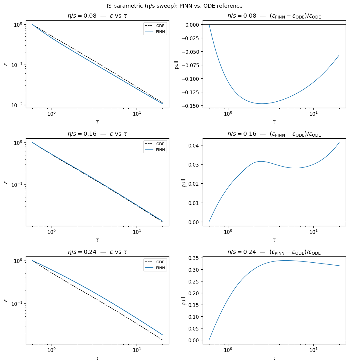FIXME caption — pulls $(\varepsilon_\theta - \varepsilon_{\text{ODE}})/\varepsilon_{\text{ODE}}$ vs $\tau$ for several $\eta/s$ values from the parametric IS run, showing accuracy is preserved across the conditioning range.

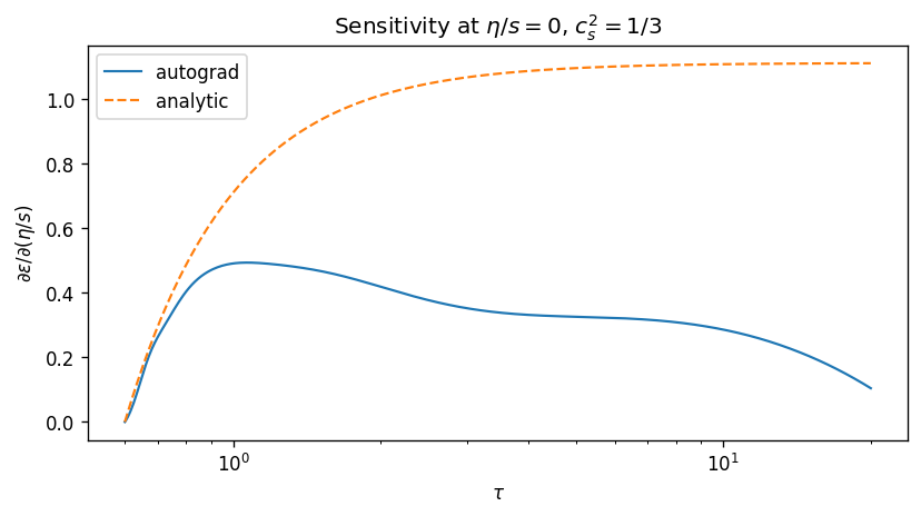FIXME caption — autograd $\partial\varepsilon/\partial(\eta/s)$ at $\eta/s = 0$ compared to the analytic first-order viscous correction. Held-out values shown as open markers.

Parameterized EoS

Stub. Same conditional architecture but now $\lambda$ includes EoS parameters. Two specific cases:

1. Constant $c_s^2$. $\lambda = (c_s^2, \eta/s)$. Used as the warm-up for joint inference (Stage 3) and as the EoS-agnostic test in Stage 1.6.5.
2. TanH-transition. A QCD-motivated crossover EoS with $c_s^2(\varepsilon) = \mathrm{sigmoid}((\varepsilon^{1/4} - \varepsilon_c^{1/4})/w)$, three parameters $(c_{\text{low}}, \varepsilon_c, w)$. Stand-in for a confinement transition without committing to the full lattice EoS.

The point of this section is to show that the inverse machinery works on a low-dimensional, physically interpretable parameter vector before generalizing to the function-space inverse problem of the next subsection.

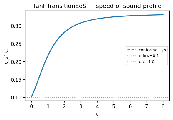FIXME caption — $c_s^2(\varepsilon)$ for the TanH-transition EoS used in the parametric inference test, with truth parameters $(c_{\text{low}} = 0.10,\, \varepsilon_c = 1.0,\, w = 0.3)$.

Neural EoS

Stub. Replace the parametric form $p(\varepsilon; \lambda)$ with a learned $p_\phi(\varepsilon)$, a small MLP with weights $\phi$ co-trained alongside the PINN. The EoS network is constrained by construction to produce physically admissible $c_s^2(\varepsilon)$: I use the Route-B parametrization $c_s^2 = \mathrm{sigmoid}(\mathrm{NN}(\log\varepsilon))$, with $p$ recovered by quadrature, which guarantees $c_s^2 \in (0,1)$ and monotone $p(\varepsilon)$ at no extra cost.

The training loss adds the data term against synthetic trajectories generated from an external truth EoS (TanhTransition or HotQCD lattice) and soft physical priors (causality, stability, conformal limit at high $\varepsilon$).

Closed-loop variant. A separate run derives $T(\varepsilon)$ thermodynamically from the learned $c_s^2$ and $p$, with a single learnable anchor $\log T_{\text{ref}}$ fixing the absolute scale. Everything else is self-consistent. This is the version with no truth leakage and is the one used for the headline EoS-recovery figure.

Numbers from the runs. HotQCD closed-loop: $p_{\text{rel,max}} = 6.8\times 10^{-3}$, $T_{\text{rel,mean}} = 1.6\times 10^{-2}$, $T_{\text{ref}}$ recovered at $184\,\text{MeV}$ (truth $\approx 190\,\text{MeV}$). Even a single trajectory at fixed $(\eta/s, \varepsilon_0)$ over-determines the EoS along the visited $\varepsilon$ range when the closed-loop priors are enforced.

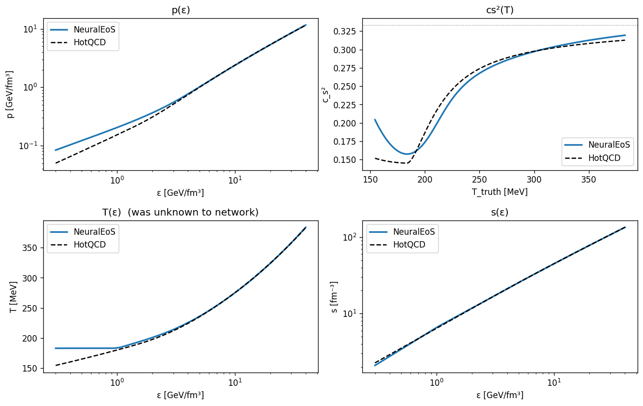FIXME caption — learned $p_\phi(\varepsilon)$, $c_s^2(\varepsilon)$, and $T(\varepsilon)$ vs HotQCD truth (Huovinen-Petreczky s95p-v1). Closed-loop run, no truth leakage on $s(\varepsilon)$.

Stage 3: Inference

Setup

Stub. Forward problem: PINN trained on the equations. Inverse problem: fix the trained PINN, and use it as a differentiable forward map to fit observed (synthetic) data and recover the underlying physical parameters with calibrated uncertainty.

Pipeline.

1. Synthetic data generated from an independent stiff-ODE reference (not from the PINN), to guarantee the forward map and ground truth are not the same object. Noise added as Gaussian with $\sigma_i = (\sigma/\varepsilon)\cdot \varepsilon_{\text{ODE}}(\tau_i)$ at $\sim 20$ log-spaced sample times.
2. Likelihood $\ell(\lambda) = -\tfrac{1}{2}\sum_i [\varepsilon_{\text{obs}}(\tau_i) - \varepsilon_\theta(\tau_i; \lambda)]^2 / \sigma_i^2$. Differentiable in $\lambda$ via autograd through the trained PINN.
3. MLE by gradient ascent (or Newton; the Hessian is also autograd). Uncertainty by Laplace / Fisher: $\mathrm{Var} \approx -1/\ell’’$ at the MLE for scalar $\lambda$, or covariance $\approx F^{-1}$ for vector $\lambda$ with $F_{ij} = -\partial^2\ell/\partial\lambda_i \partial\lambda_j$.
4. Calibration via repeated noise realizations ($N \ge 200$): the pull histogram and empirical 68% / 95% coverage are the actual validation. A recovered point estimate alone proves nothing.

The PINN itself is not retrained for inference. Data enters only at the inference layer, never in the PINN training loss.

Scalar inverse: $\eta/s$ extraction

Numbers from the runs.

• Conformal: $\mathrm{pull_mean} = -0.023$, $\mathrm{pull_std} = 0.998$, $\mathrm{coverage}_{68} = 0.650$.
• Non-conformal: $\mathrm{pull_mean} = -0.017$, $\mathrm{coverage}_{68} = 0.670$.

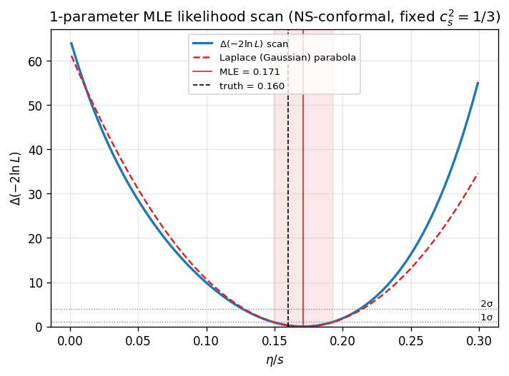1-parameter likelihood scan $\Delta(-2\ln L)$ vs $\eta/s$ for a single noise realization (conformal NS, fixed $c_s^2 = 1/3$). The Laplace parabola (dashed) tracks the true scan closely, indicating the Gaussian approximation is adequate at this noise level. MLE $= 0.171$, truth $= 0.160$; the $1\sigma$ interval is shown shaded.

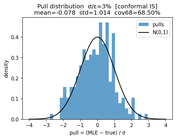Pull histogram for $\eta/s$ extraction over 200 noise realizations at $\sigma/\varepsilon = 3\%$, with the standard normal overlaid. Pull mean $= -0.023$, pull std $= 0.998$.

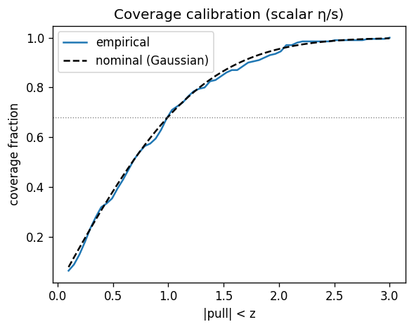Empirical coverage vs nominal for the scalar $\eta/s$ extraction. Empirical $68\%$ coverage $= 0.650$, consistent with the calibrated interval.

Joint inverse: $(c_s^2, \eta/s)$ degeneracy

Stub. Generalize from scalar to vector $\lambda$. Fisher matrix via the autograd Hessian; eigendecomposition exposes the conditioning of the inverse problem. The expected and reportable result is a partial degeneracy between $c_s^2$ and $\eta/s$ along a single Bjorken trajectory: both modulate the cooling rate, and Fisher has a flat eigendirection in $(c_s^2, \eta/s)$ space.

Numbers from the run. Condition number $\approx 163$. The Fisher 68% ellipse covers $> 99\%$ of the physical range along the flat eigendirection. This is the quantitative motivation for moving to Gubser flow, where the richer geometry breaks the degeneracy.

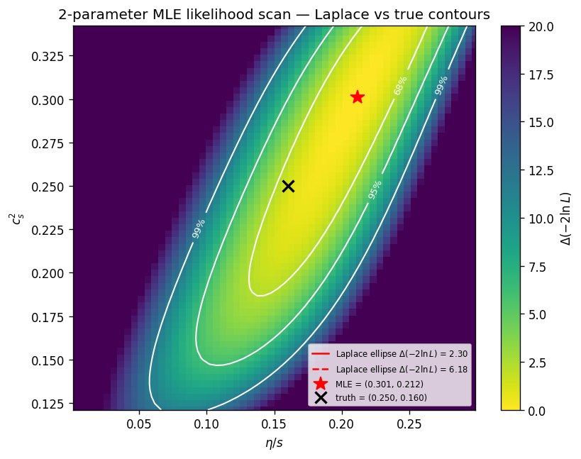2-parameter likelihood scan $\Delta(-2\ln L)$ in the $(c_s^2, \eta/s)$ plane. The true contours (colored surface) and Laplace ellipses (white, at $\Delta = 2.30$ and $6.18$ corresponding to $68\%$ and $95\%$ in 2 parameters) are visibly elongated along the diagonal, quantifying the degeneracy: both parameters modulate the Bjorken cooling rate in a correlated way. MLE at $(0.301, 0.212)$ (star), truth at $(0.250, 0.160)$ (cross).

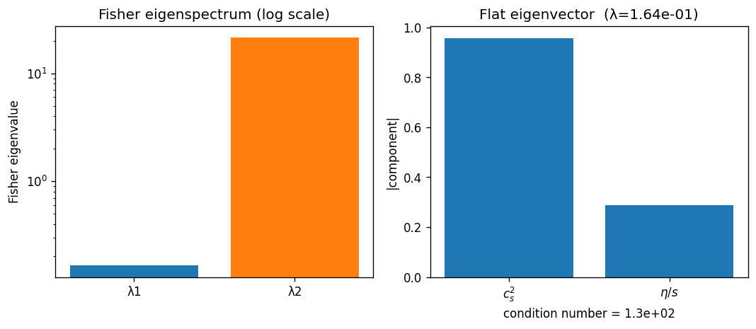Fisher eigenspectrum and the flat-direction eigenvector in $(c_s^2, \eta/s)$ space. Condition number $\approx 163$.

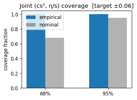Joint 68% / 95% Fisher ellipse compared to the scatter of $\hat\lambda$ over noise realizations.

Recovery of the HotQCD equation of state

Stub. The function-space inverse problem: reconstruct $p(\varepsilon)$, $T(\varepsilon)$, and $s(\varepsilon)$ from a small set of noisy trajectories. The Neural EoS architecture of Stage 2 is the forward map; here it is fit to synthetic data drawn from the Huovinen-Petreczky s95p-v1 lattice parametrization.

Pipeline. Closed-loop architecture (no $s(\varepsilon)$ leakage). Synthetic data on a $4$-event $\varepsilon_0$ grid mimicking a centrality scan, fixed $\eta/s = 0.16$. Uncertainty by ensemble: $\sim 12$ independent trainings on independent noise realizations at $\sigma/\varepsilon = 5\%$, giving 68% bands on the recovered functions.

Trace anomaly. The dimensionless QCD interaction measure $\Delta(T) = (\varepsilon - 3p)/T^4$ is the physically interesting derived quantity, exhibiting a characteristic bump at the crossover. The naive MSE-loss noise-UQ ensemble under-recovers both the peak height and its position: median peak $\Delta = 3.93$ at $T = 230\,\text{MeV}$ against truth $5.60$ at $209\,\text{MeV}$. Three fixes applied in sequence remove the bulk of the gap: (a) $\chi^2$ loss weighting instead of MSE on absolute residuals (peak height $\to 4.36$, position $\to 222\,\text{MeV}$); (b) a wider EoS-network (hidden $= 128$, depth $= 5$) restoring peak height to $5.40$ but with position drifting to $242\,\text{MeV}$; (c) low-$\varepsilon_0$ events ($\varepsilon_0 \in {1, 2}\,\text{GeV/fm}^3$) extending the probed range into the hadronic phase, which fixes the position at the cost of a small height retreat: median peak $5.18$ at $T = 222\,\text{MeV}$, height within $8\%$ and position within $6\%$ of truth.

A further variant chi2_bignet_qcd is included in the comparison panel as an additional probe of the recovery’s stability under setup changes. It overshoots the peak ($\Delta \approx 9.4$) and shifts the position downward to $T \approx 181\,\text{MeV}$, indicating that the recovery is not robust to all setup variations; the lowE configuration is the result quoted as the headline.

Bayesian variants and their failures. Two attempts to add proper Bayesian uncertainty quantification (RFF + mean-field VI; last-layer Bayes) are documented as informative negative results. The RFF basis is too rigid to fit HotQCD and the variational posterior collapses around a biased point at $T_{\text{ref}} = 217 \pm 3\,\text{MeV}$ (pull $+9.5\sigma$, miscalibrated). Last-layer Bayes centers correctly at $196 \pm 3\,\text{MeV}$ but the deterministic feature extractor absorbs the epistemic uncertainty, so coverage still under-covers. These are reported as cautionary tales for downstream extensions.

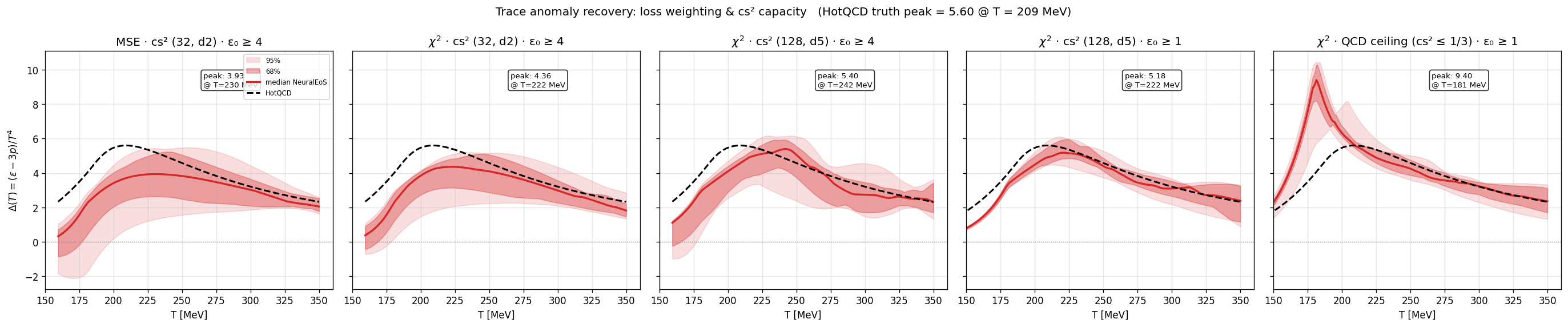FIXME caption — comparison of $\Delta(T) = (\varepsilon - 3p)/T^4$ vs HotQCD truth across loss / capacity / data fixes: MSE → $\chi^2$ loss → big-net → big-net + low-$\varepsilon_0$. The lowE panel is the headline result, with median peak within 8% of truth height and 6% in $T$. The additional chi2_bignet_qcd panel is included as a robustness probe and is described in the text.

Conclusions and future directions

Introduce idea that PINNs can be connected – indeed they don’t need to be PINNs, just NNs, where appropriate, whose derivatives are well-conditioned – to allow the gradients to flow from front to back in a more complicated analysis.

Provide an example

Other directions for future work

Appendix

Exact solutions to RHD

Bjorken mathematical details

Gubser mathematical details