Singular Value Structure of Transformer Attention Heads
Published:
Introduction
The previous post established the basic distributional facts about transformer weight matrices: the element-wise statistics of $W_Q$, $W_K$, and $W_{QK}$ across several architectures, how the trained distributions depart from their Gaussian initialization, and the amplification of non-Gaussianity in the matrix product $W_{QK} = W_Q^T W_K$. Those results characterized the marginal, element-wise statistics of these matrices. This post moves to the spectral structure: the singular value decomposition of $W_{QK}$, which captures the geometry of the learned attention patterns rather than just the distribution of individual matrix elements. The interactive dashboard linked above allows exploration of these distributions across models, layers, and heads directly.
Throughout this post, GPT-2 ($d = 768$, $n_h = 12$, $d_h = 64$) serves as the primary illustration. Cross-model comparisons appear in the final section. All spectral quantities are expressed in terms of eigenvalues $\lambda_k = \sigma_k^2$, where $\sigma_k$ are the singular values from the SVD of $W_{QK}$. This convention aligns naturally with the Marchenko-Pastur distribution, which is stated as a density over eigenvalues.
Recall that $W_{QK}$ is a $d \times d$ matrix of rank at most $d_h = d/n_h$, where $d_h$ is the head dimension. Its eigenvalues ${\lambda_k}$ define the effective interaction strengths in the attention logit computation; in a physics context, these are the mode energies of the coupling matrix. The distribution of these modes—whether concentrated in a few dominant directions or spread across many—encodes how many effective degrees of freedom each attention head uses and how the learned attention geometry differs from the random-matrix baseline.
The random-matrix expectations were developed in the previous post: for $W_{QK}$ constructed from Gaussian $W_Q$ and $W_K$, the eigenvalue spectrum follows a gapped Marchenko-Pastur (MP) distribution with $d_h$ nonzero values. The MP distribution describes the eigenvalue density of Wishart matrices $W W^T$; here the relevant object is $W_{QK} W_{QK}^T = W_Q^T W_K W_K^T W_Q$, and its eigenvalues are the squares of the singular values of $W_{QK}$.
Any departure from this baseline in trained models is, by construction, a signal of learned structure. To make this comparison more rigorous, Monte Carlo simulations of random matrices were used to generate the appropriate matrix ensemble given the GPT-2 architecture parameters. These results are described in more detail in a future post on random matrix theory baselines; here we use the simulations to sharpen quantitative expectations.
The simulated eigenvalue distribution is shown below using $d = 768$ and $d_h = 64$. These results assume an underlying Gaussian element-wise standard deviation of $\sigma = 1$. While the spectrum shares the essential shape of the Marchenko-Pastur distribution, the empirical distribution is somewhat wider: the product structure of $W_{QK} = W_Q^T W_K$ introduces fourth-order moments that shift the spectral edge relative to the naive MP prediction for a single matrix. For some statistics, a moment-method product expansion provides analytical corrections; those results are also shown and agree well with the simulations.
Eigenvalue Distributions
Single-Head Spectra
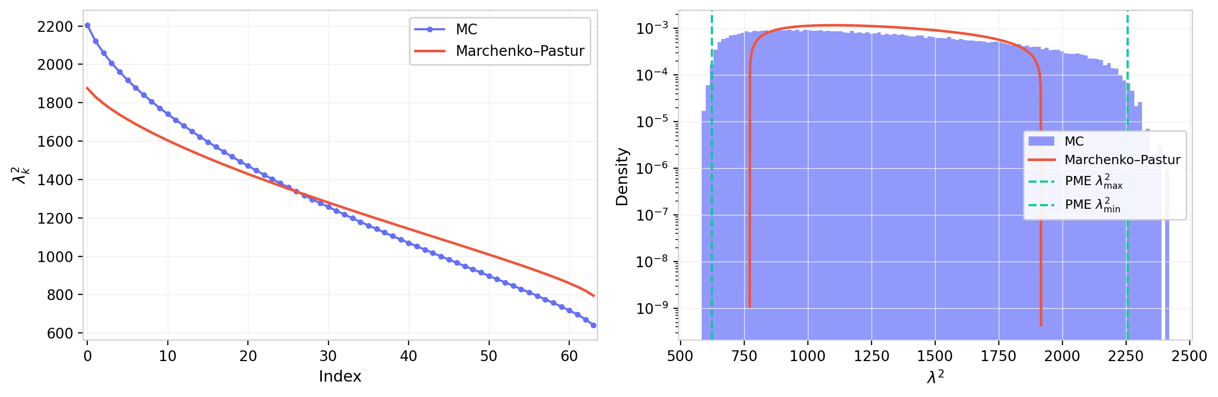
Figure 1: Eigenvalue distribution from Monte Carlo simulation of the random-matrix baseline (GPT-2 dimensions, $d=768$, $d_h=64$). Left: full distribution with Marchenko–Pastur density overlay and bounds. Right: zoom on the upper edge showing MC support beyond the MP limit, well-captured by the analytical moment-method calculation.
Figure 1 establishes the baseline against which trained models are compared. The simulated distribution broadly follows the MP shape but with a heavier upper tail: the product structure of $W_{QK}$ shifts the spectral edge beyond the naive MP bound, an effect captured quantitatively by the moment-method calculation. This correction is modest in absolute terms but matters when identifying whether the largest eigenvalues of a trained head represent genuine learned structure or merely exceed the MP bound due to the product geometry.
To ground these expectations against trained models, we compare two specific attention heads that illustrate the range of spectral behavior. The first has an eigenvalue spectrum that closely follows the random-matrix baseline; the second exhibits clear outlier eigenvalues emerging from the bulk. Note that for heads with very large leading eigenvalues, the linear scale can compress the bulk and obscure the spectral gap; this is worth bearing in mind when interpreting the right panel.
The blue head shows a clear excess at low index: the largest eigenvalues are substantially larger than in the other head, which directly contributes to the points in the right panel that lie outside the bulk. The kinks near index $= 4$ and $d_h$ delineate the bulk, and the slope of the distribution in that region determines the curvature of $P(\lambda)$. The peak at $\lambda = 0$ corresponds to the $d - d_h$ zero eigenvalues imposed by the low-rank structure of $W_{QK}$.
The red head exhibits a tighter bulk with only marginal deviations at the upper edge. Both heads retain a spectral gap. For some heads this gap closes, and the distribution transitions toward a power-law falloff; examples appear in the full-model heatmaps below.
An MP-like head, in physical terms, is one whose attention geometry is consistent with random initialization: the modes are approximately degenerate and no direction in the $d_h$-dimensional subspace has been singled out by training. An outlier eigenvalue, by contrast, indicates that training has identified and reinforced a specific direction in query-key space, concentrating attention logit strength along that mode.
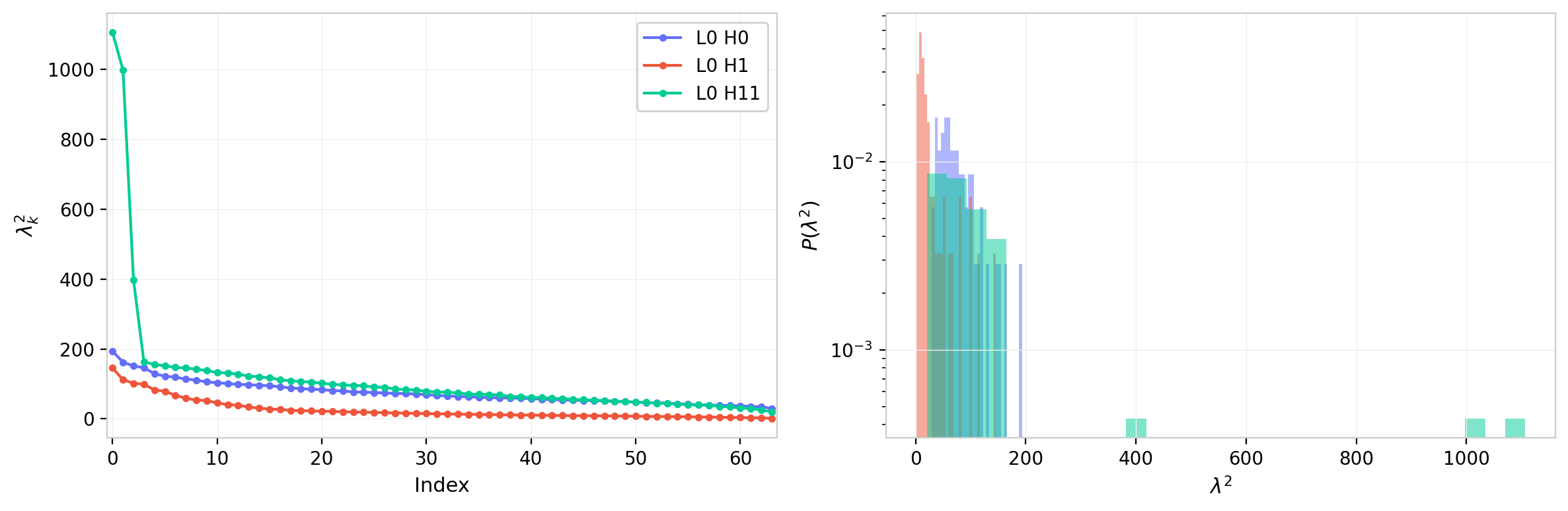
Figure 2: Eigenvalue spectra for two GPT-2 attention heads. Left: eigenvalues $\lambda_k$ vs. index. Right: eigenvalue density $P(\lambda)$, log scale. The MP-like head (L7 H6, blue) closely follows the random-matrix baseline; the outlier head (L1 H0, red) shows dominant low-rank structure with eigenvalues well above the bulk.
Spectra Across the Full Model
To summarize the spectral structure across the full model, the figures below show the $W_{QK}$ eigenvalues for every attention head as 2D heatmaps with layer and head on the vertical axis.
The largest eigenvalues are concentrated in the earliest layers, reaching values $\lambda_{\max} \lesssim 50$ for some heads in layer 0. These early-layer heads also tend to show a steeper index profile, with smaller values of $\lambda_{\min}$, indicating a higher condition number and more pronounced spectral hierarchy. The layer dependence is not monotone: several intermediate layers show renewed growth in the leading eigenvalue, hinting at distinct functional regimes across the network depth.
The eigenvalue density heatmap makes the gap structure more legible. Most heads retain a clear gap between the bulk and the zero eigenvalues, confirming that the low-rank constraint is respected and no spurious rank inflation has occurred. A minority of heads, primarily in the earliest layers, show the gap closing and the distribution broadening into a more power-law-like tail. Head-to-head variation within a given layer is substantial, suggesting that heads within the same layer develop qualitatively different attention geometries.
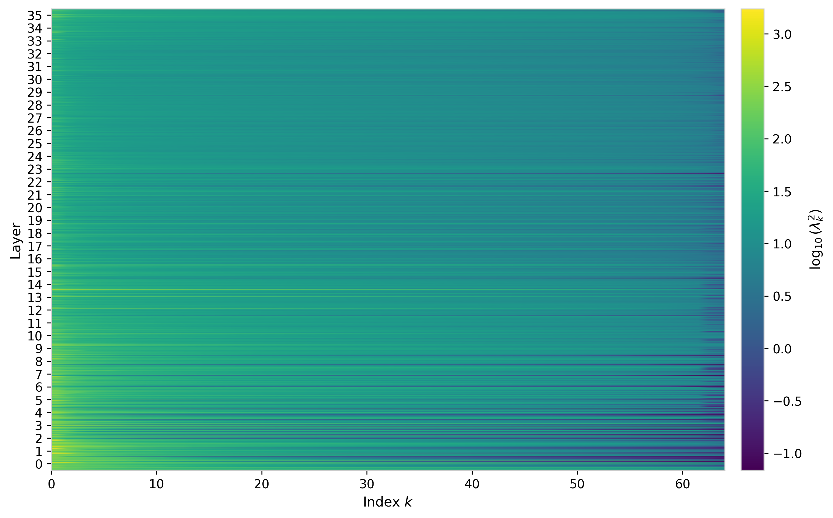
Figure 3: Eigenvalues $\lambda_k$ vs. index across all attention heads in GPT-2, shown as a heatmap on log color scale. Each row is one head, grouped by layer. Early layers show the largest leading eigenvalues and steepest index profiles.
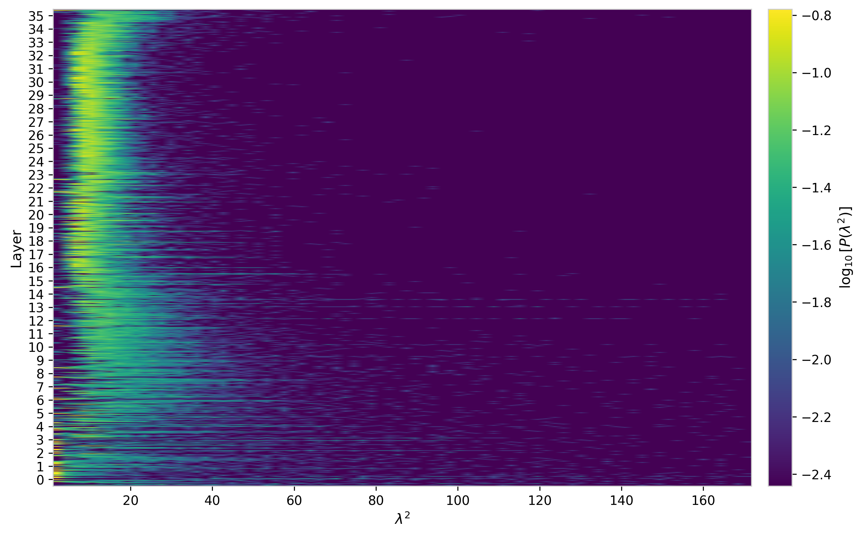
Figure 4: Eigenvalue density $P(\lambda)$ across all attention heads in GPT-2, log color scale. Color scale is set to exclude the zero-bin peak. Variation in bulk width and gap size is apparent both across layers and across heads within a layer.
Per-Head Distributions
The per-head grid provides a closer look at the spectral diversity within a single layer.
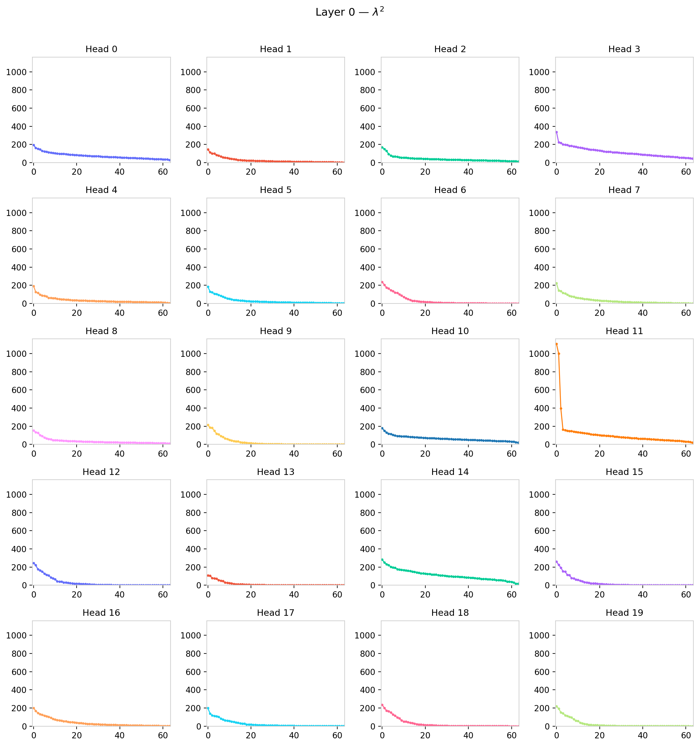
Figure 5: Eigenvalues $\lambda_k$ vs. index for all 12 attention heads in GPT-2 layer 0.
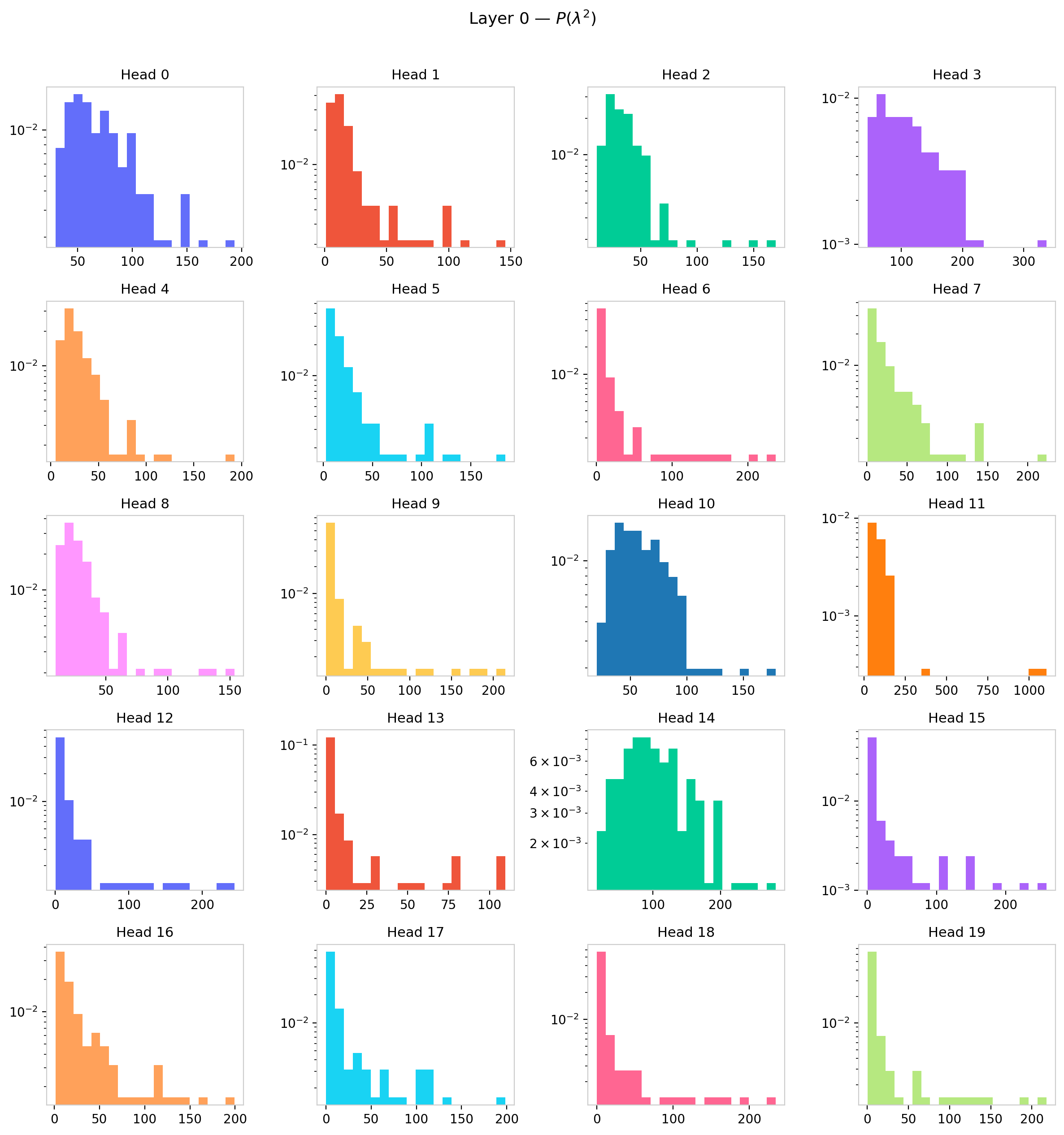
Figure 6: Eigenvalue density $P(\lambda)$ for all 12 attention heads in GPT-2 layer 0. Heads develop qualitatively different spectral shapes within the same layer, suggesting distinct functional roles.
Within a single layer, the heads span a striking range of spectral shapes. Some heads retain a compact, nearly uniform bulk with a clear gap—close to the random-matrix baseline. Others exhibit one or two dominant eigenvalues well above the bulk, indicating that those heads have learned to concentrate attention along a low-dimensional direction in query-key space, effectively reducing their functional rank below $d_h$. A few heads show an intermediate regime: a bulk that has broadened and begun to merge with the outlier region, erasing the gap. This diversity within a layer argues against treating all heads as functionally equivalent and motivates the per-head statistical summaries developed in the next section.
Eigenvalue Statistics
The full eigenvalue spectrum contains $d_h$ values per head. To track how spectral structure varies across layers and models, we compress these into scalar summary statistics.
Leading Eigenvalue
The leading eigenvalue $\lambda_0$ sets the overall scale of the attention logits for each head. Its variation across layers reflects the model’s allocation of attention strength across depth. The layer average decreases through approximately the first half of the network ($\sim$layer 18 for this model), then flattens with a possible mild upturn in the final layers—a trend present in other statistics, including the element-wise standard deviation, and reproduced across model families. The head-to-head spread within each layer is substantial, consistent with the qualitative diversity visible in the per-head grids.
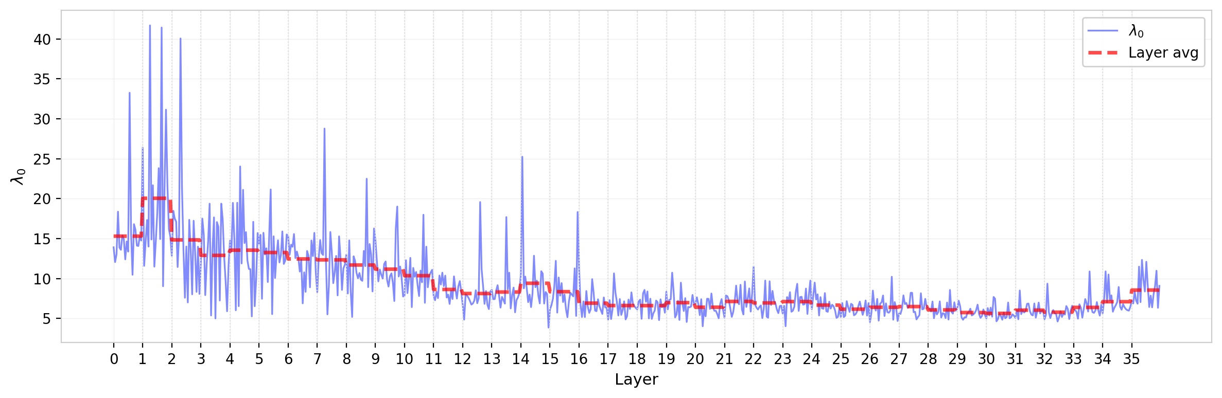
Figure 7: Leading eigenvalue $\lambda_0$ of $W_{QK}$ across all attention heads in GPT-2, ordered by layer. Dashed red line shows layer average. The layer average decays through the first half of the network before flattening.
Participation Ratio and Normalized Participation Ratio
The participation ratio $\text{PR} = (\sum_k \lambda_k)^2 / \sum_k \lambda_k^2$ measures how many eigenvalues contribute meaningfully to the spectrum. For a flat spectrum (all $\lambda_k$ equal), $\text{PR} = d_h$; for a single dominant mode, $\text{PR} = 1$. The normalized participation ratio $\text{NPR} = \text{PR}/d_h$ maps this to $[0, 1]$. Because the Monte Carlo prediction for NPR is independent of the underlying element-wise $\sigma$, it provides a cleaner comparison to the random-matrix baseline than the leading eigenvalue.
For GPT-2, NPR is relatively high across most heads—close to the random-matrix prediction—indicating that training has not dramatically reduced the effective rank of most attention heads. The layer dependence is mild but present, with a modest decrease toward the network’s middle layers; the trend reverses in the final layers, where a slight increase in NPR is observed. This is consistent with the picture from the leading eigenvalue: early layers develop the most prominent outlier modes, while later layers retain a more democratic eigenvalue distribution.
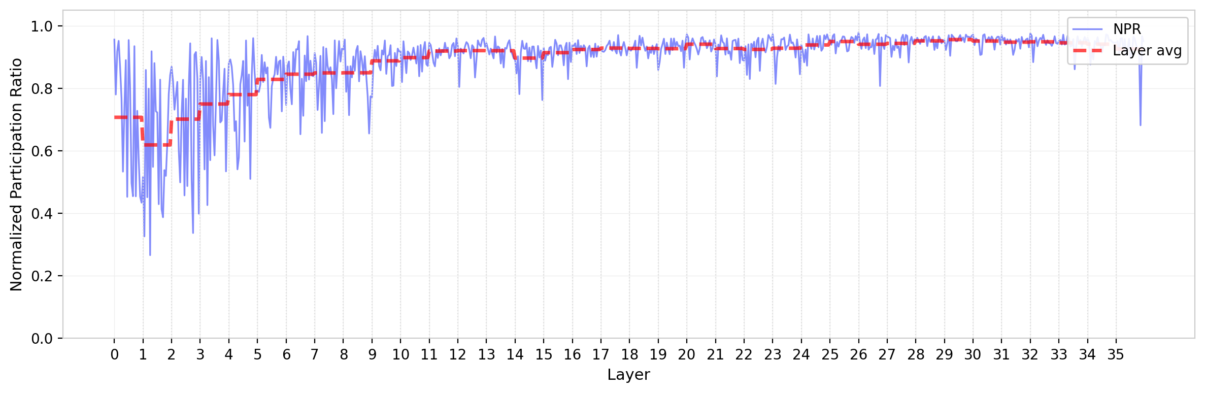
Figure 8: Normalized participation ratio of $W_{QK}$ eigenvalues across all attention heads in GPT-2. Dashed red line shows layer average. NPR remains near the random-matrix prediction for most heads, with modest layer dependence.
Spectral Entropy
The spectral entropy $S_\lambda = -\sum_k p_k \ln p_k$, where $p_k = \lambda_k / \sum_j \lambda_j$, provides a related but distinct measure of spectral concentration. While the participation ratio counts effective modes, the entropy is more sensitive to the shape of the distribution across those modes—in particular, to whether the eigenvalue weight is distributed smoothly or has sharp peaks.
The spectral entropy tracks the NPR qualitatively but is not redundant: heads with the same NPR can differ in entropy if their eigenvalue weights are distributed differently within the bulk. In practice the two statistics are strongly correlated for GPT-2, suggesting that for this model the spectral shape is well-characterized by either measure. The layer dependence of the entropy mirrors that of the NPR, with the highest entropies (most diffuse spectra) in later layers and the lowest (most concentrated) in early layers.
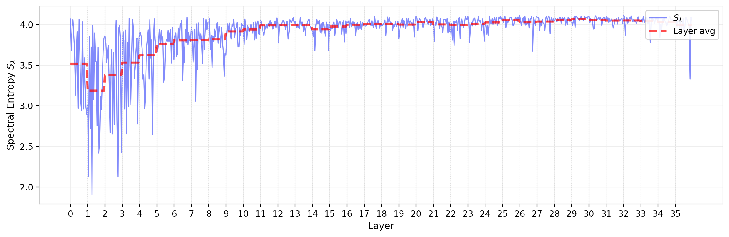
Figure 9: Spectral entropy $S_\lambda$ of $W_{QK}$ eigenvalues across all attention heads in GPT-2. Dashed red line shows layer average. The layer dependence mirrors the NPR, with lower entropy (more concentrated spectra) in early layers.
Condition Number
The condition number $\kappa = \lambda_{\max} / \lambda_{\min}$ (computed over the $d_h$ nonzero eigenvalues) measures the dynamic range of the spectrum. A condition number near 1 indicates a flat, democratic spectrum; large values indicate that some modes are orders of magnitude stronger than others. For GPT-2, typical condition numbers are modest—on the order of 4 for most heads—consistent with the high NPR values observed above. The early-layer outlier heads push the distribution upward, but GPT-2’s condition numbers remain well-behaved compared to some larger models where $\kappa$ reaches dramatically higher values (see the cross-model comparison below).
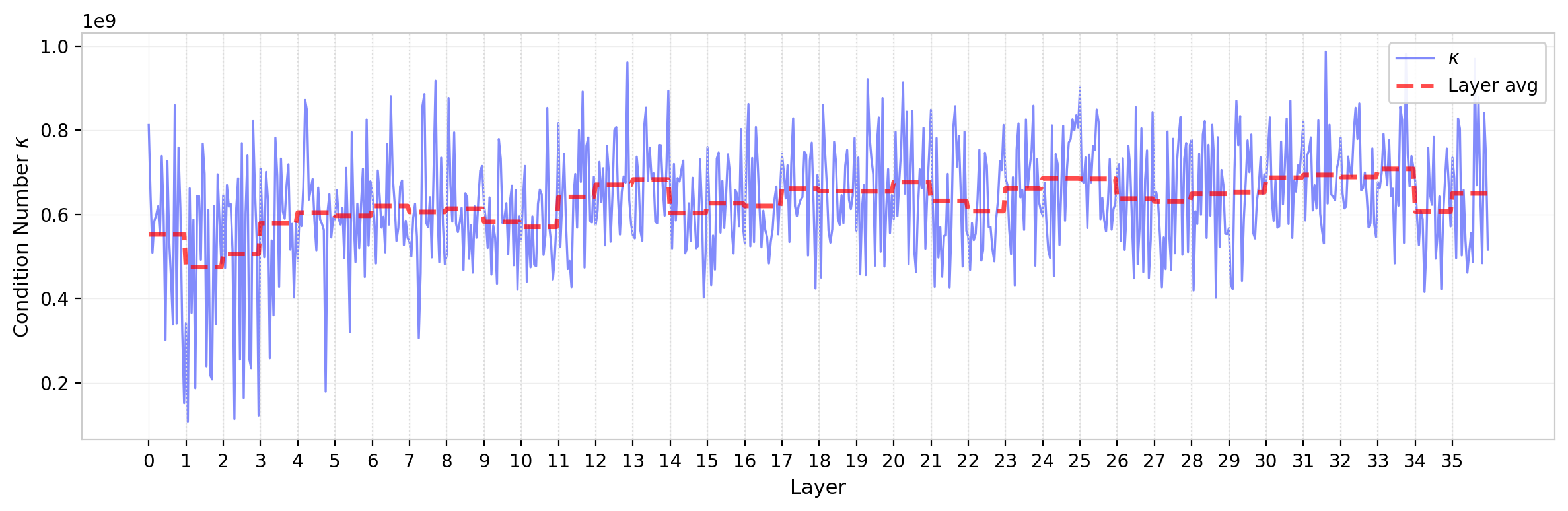
Figure 10: Condition number $\kappa$ of $W_{QK}$ eigenvalues across all attention heads in GPT-2 (log scale). Dashed red line shows layer average. Most heads cluster near $\kappa \sim 4$, with early-layer heads showing larger values.
Entropy vs. Participation Ratio
The relationship between spectral entropy and the normalized participation ratio provides a consistency check: both measure spectral concentration, but weight the tails differently.
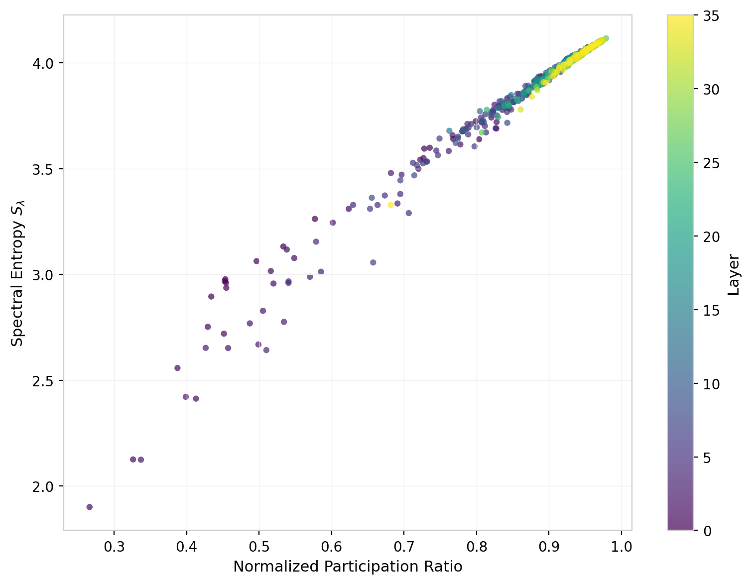
Figure 11: Spectral entropy vs. normalized participation ratio for all GPT-2 attention heads, colored by layer.
The two measures are strongly correlated, tracing a tight curve through the joint space. The heads with the lowest NPR and entropy are predominantly from early layers (darker colors), confirming that spectral concentration is a layer-dependent property rather than random variation. The scatter around the main trend is modest, indicating that for GPT-2, NPR and spectral entropy are largely redundant as characterizations of spectral shape; a single measure suffices for most purposes. This may not hold for other architectures where the eigenvalue distribution takes qualitatively different forms.
Correlations with Element-Wise Statistics
The singular value statistics developed above characterize the spectral geometry of $W_{QK}$; the element-wise statistics from the previous post characterize its marginal distribution. These are not independent descriptions. The standard deviation $\sigma$ sets the overall scale of the matrix elements and therefore controls the scale of the singular values. The question is how much of the spectral structure is determined by $\sigma$ alone, and how much is independent.
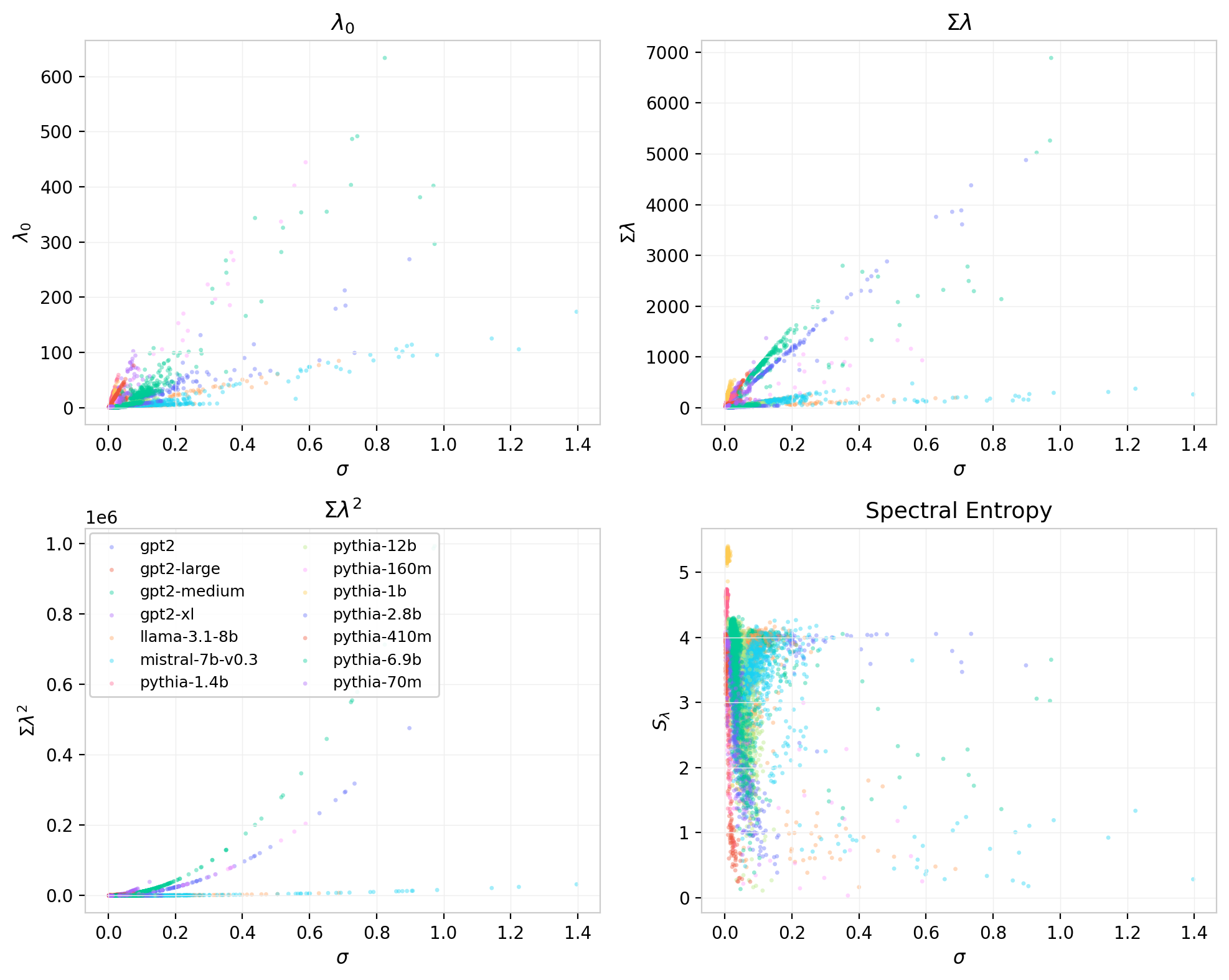
Figure 12: Eigenvalue statistics vs. element-wise $\sigma$ for all attention heads across models. Top left: $\lambda_0$ (approximately linear with substantial scatter). Top right: $\sum\lambda_k$ (linear). Bottom left: $\sum\lambda_k^2$ (quadratic, tightest relationship). Bottom right: spectral entropy.
As expected, $\sigma$ is the dominant driver of the overall eigenvalue scale. The relationship between $\sigma$ and $\sum \lambda_k^2$ is the tightest, reflecting the fact that
\[\sum \lambda_k^2 = \|W_{QK}\|_F^2 = \text{tr}(W_{QK}^T W_{QK})\,,\]which is determined directly by the element-wise variance. The leading eigenvalue $\lambda_0$ is more scattered: heads with similar $\sigma$ can differ substantially in how concentrated the spectrum is. Spectral entropy shows no strong dependence on $\sigma$, which is consistent with NPR being approximately $\sigma$-independent in the random-matrix ensemble. Together these results suggest that $\sigma$ accounts for the bulk of the spectral scale, while the shape statistics (entropy, NPR, condition number) capture orthogonal variation in how that energy is distributed across modes.
Cross-Model Comparison
The GPT-2 results establish a baseline. Extending the analysis to the Pythia suite and to LLaMA and Mistral reveals both robust patterns and striking architecture-dependent anomalies.
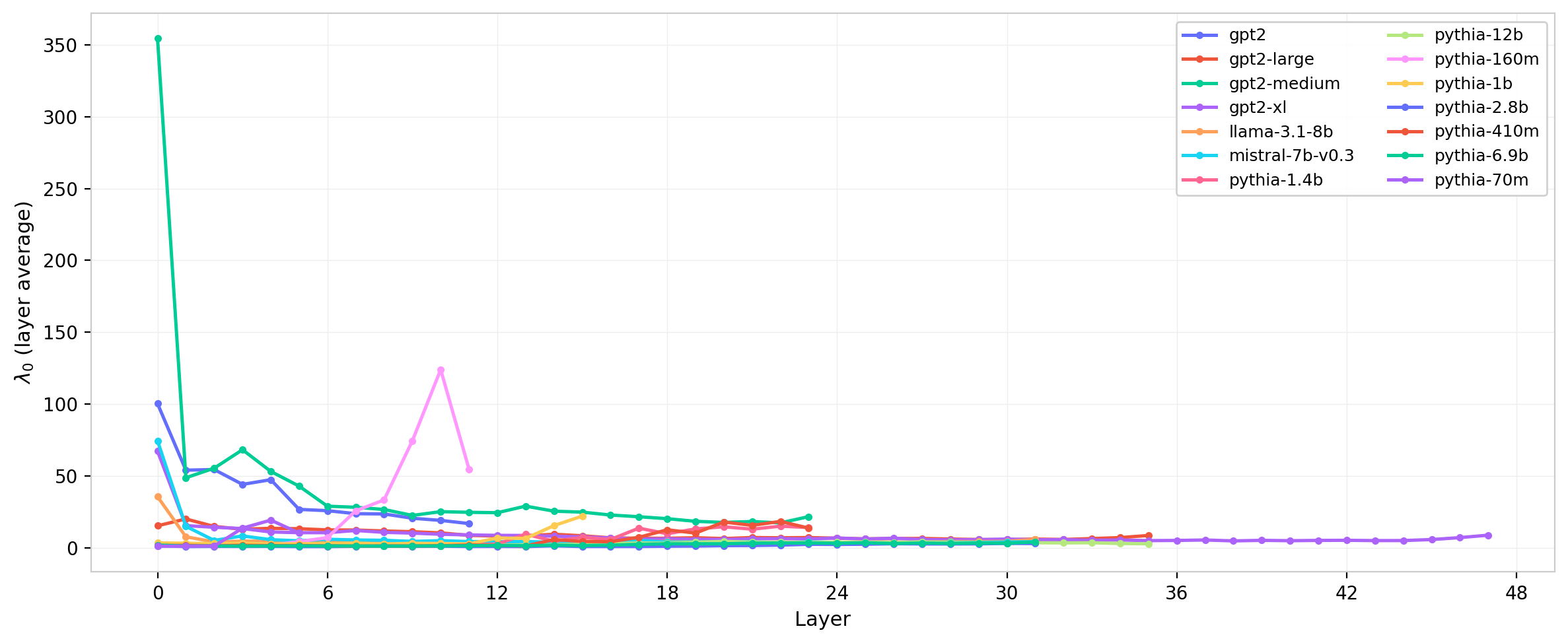
Figure 13: Leading eigenvalue $\lambda_0$ (layer-averaged) across layers for several model families.
The leading eigenvalue profiles are broadly similar in shape across families—largest in early layers, decaying through the middle of the network—but differ substantially in absolute scale. The Mistral/LLaMA sigma anomaly identified in the previous post (a $\sim$5–10$\times$ difference in element-wise $\sigma$ attributable to different attention normalization conventions) propagates directly into the eigenvalue scale, as expected from the quadratic $\sigma$-dependence of $\sum \lambda_k^2$. The leading eigenvalue difference across those two families is consistent with this explanation.
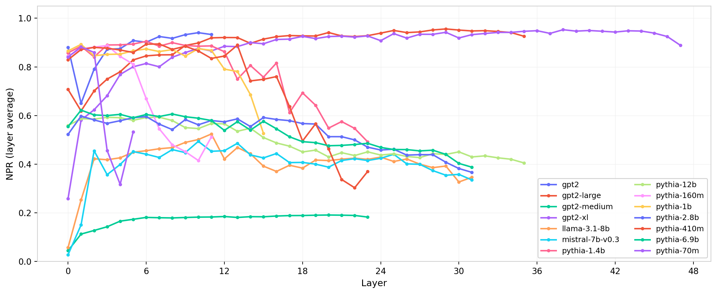
Figure 14: Normalized participation ratio (layer-averaged) across layers for several model families.
NPR reveals a clear trend with model scale. Smaller models (GPT-2, smaller Pythia variants) show NPR values close to the random-matrix prediction, while larger models exhibit systematically lower NPR. This indicates that larger models have learned more concentrated attention geometries—fewer effective modes per head—consistent with greater functional specialization as model capacity increases. The Pythia suite, with its range of scales from 70M to 12B parameters, makes this trend particularly legible.
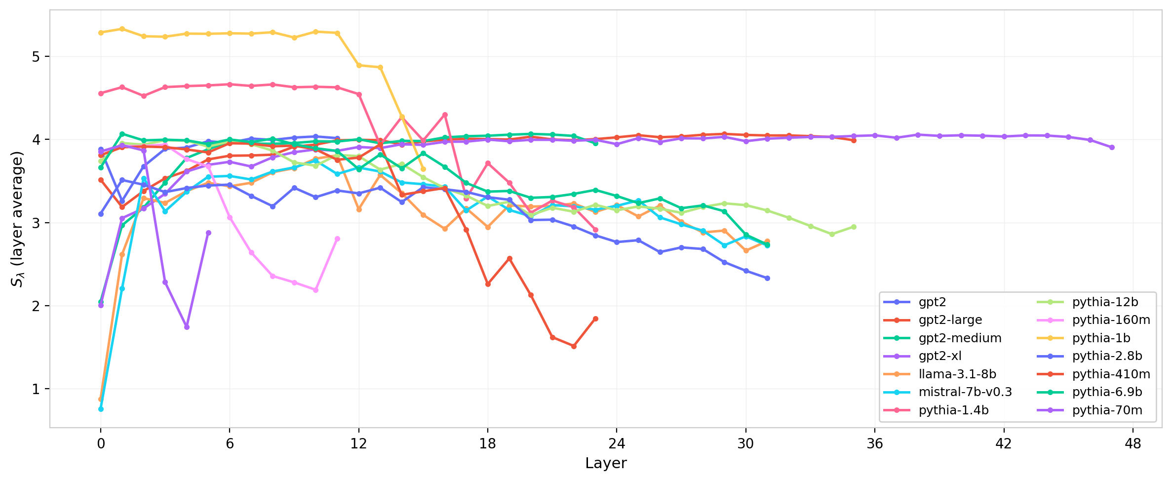
Figure 15: Spectral entropy $S_\lambda$ (layer-averaged) across layers for several model families.
Spectral entropy tells a consistent story: larger models have lower entropy (more concentrated spectra), and the layer profile sharpens with scale. The entropy differences between model families are larger than the within-family layer variation for the largest models, suggesting that the spectral shape is more strongly determined by model scale than by depth position for those models.
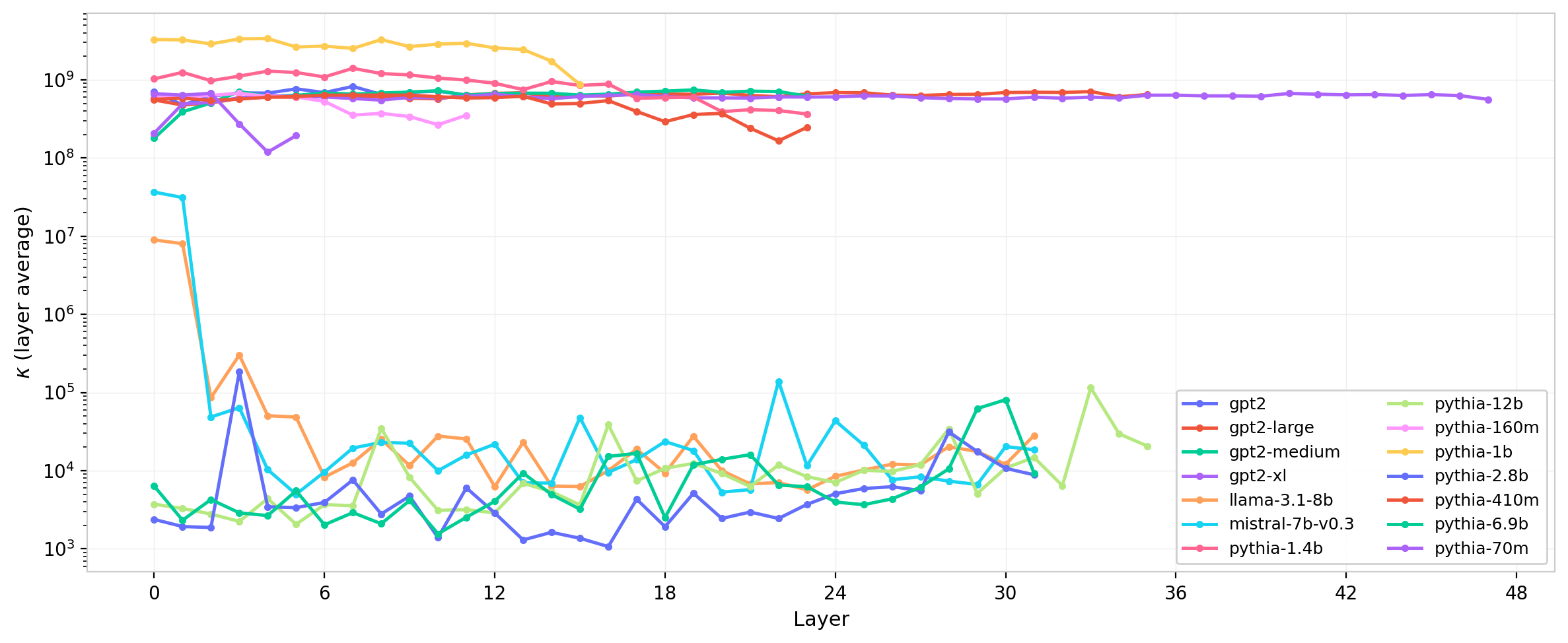
Figure 16: Condition number $\kappa$ (layer-averaged, log scale) across layers for several model families.
The condition number exhibits the most dramatic cross-model variation of any statistic considered here. GPT-2 remains well-conditioned ($\kappa \sim 4$). Some larger models, including GPT-2 medium and certain Pythia checkpoints, show condition numbers orders of magnitude larger. The most extreme cases—where $\kappa$ reaches into the millions—suggest the presence of nearly degenerate small eigenvalues: modes that are nominally nonzero but effectively inert. Whether these represent numerical artifacts of the low-rank structure, dead attention directions, or a genuine feature of the learned representation is an open question that warrants direct inspection of the smallest eigenvalue modes in those heads.
Discussion
The central result is that the spectral structure of $W_{QK}$ is neither random nor trivially structured: it sits between the Marchenko-Pastur baseline and a maximally low-rank extreme, with the position in that spectrum depending on layer depth, head identity, and model scale.
High NPR, close to the random-matrix prediction, means that a head uses nearly all $d_h$ available dimensions of the query-key interaction space. No single direction dominates; the attention logit is distributed across many modes of roughly similar strength. In a physics picture, this is analogous to a disordered coupling matrix with many nearly degenerate energy levels—the attention pattern it generates will be diffuse and sensitive to the full geometry of the input rather than to any single feature direction. For GPT-2, most heads are in this regime, which may explain why the model’s attention patterns are notoriously difficult to interpret: there is simply no single dominant direction to point at.
Lower NPR in larger models indicates that training has identified and reinforced a smaller number of directions in the query-key space. Each head is effectively operating with a lower-dimensional interaction geometry. This is consistent with the hypothesis that larger models develop more specialized, lower-rank attention heads—heads that respond selectively to particular structural features of the input rather than integrating broadly across the residual stream. The participation ratio provides a scalar measure of this specialization that is independent of the overall eigenvalue scale.
The connection to element-wise non-Gaussianity from the previous post is indirect but real. The element-wise $\sigma$ controls the overall spectral scale, accounting for the bulk of the variance in $\sum \lambda_k^2$. But the shape statistics—NPR, spectral entropy, condition number—carry orthogonal information. Heads with unusually large leading eigenvalues or anomalously low NPR tend to be the same heads that showed the most pronounced non-Gaussianity in the element-wise distributions: early-layer heads with heavy tails or asymmetric $W_{QK}$ distributions. The spectral and element-wise measures are therefore correlated indicators of the same underlying phenomenon—learned, structured departures from random initialization—but neither fully subsumes the other.
The most anomalous heads in both frameworks are the early-layer outliers with dominant leading eigenvalues, low participation ratios, and high condition numbers. These heads appear to have developed strongly directional attention geometries early in training and maintain them through the network. Whether this reflects a specific computational function—attending to syntactic heads, positional structure, or other early-layer features—is a question that the eigenvalue decomposition alone cannot answer; it motivates connecting the spectral structure to attention pattern visualization and probing tasks.
What Comes Next
The analyses here are static snapshots of trained models. A natural follow-up is to ask how the eigenvalue structure develops over the course of training. The Pythia suite provides an unusual resource for this: 154 checkpoints spanning pretraining, enabling the spectral statistics to be tracked continuously rather than inferred from final weights alone. The next post examines this temporal dimension—how NPR, leading eigenvalue, and condition number evolve across training steps, whether different heads develop their spectral structure on different timescales, and whether the anomalous initialization structure identified in the element-wise distributions leaves a detectable imprint on the spectral evolution.
The code, data, and interactive dashboards for reproducing and extending this analysis are available at the links above.