Training Dynamics of Transformer Attention Heads

Introduction

The previous posts in this series characterized the weight matrix statistics and spectral structure of $W_{QK}$ in trained models: how the element-wise distributions depart from Gaussian initialization, how the singular value spectra of attention heads vary across layers, and how summary statistics like the stable rank and condition number scale with model size. Those analyses were snapshots of final, trained weights. This post studies how these weights evolve throughout the training process.

The Pythia model suite provides an unusual resource for this: a set of models spanning 70M to 12B parameters, each with approximately 154 publicly released checkpoints taken at regular intervals across pretraining on the Pile. Rather than inferring training history from the endpoint, these checkpoints allow the spectral statistics of $W_{QK}$ to be tracked directly as a function of training step. The reference model throughout is Pythia-1.4B ($d = 2048$, $n_h = 16$, $d_h = 128$, 24 layers), which is large enough to exhibit diverse head behavior.

The central questions are: when during training does the spectral structure of $W_{QK}$ consolidate? Do different heads converge on their final geometry at different rates? And does the layer-dependent organization identified in the static analysis (e.g. early layers developing the most concentrated spectra),emerge early in training or gradually across the full pretraining horizon?

The interactive dashboard linked above supports direct exploration of these statistics across the Pythia suite.

Basic Results

Element-Wise Distributions Across Training

The element-wise statistics of $W_{QK}$ evolve substantially during the early phase of training and then stabilize. The figure below shows the two-dimensional distribution of matrix elements at a fixed head and layer for four different heads, chosen as exemplars of different behaviors observed in the data. The upper left panel shows a head with a relatively narrow weight distribution, with a width that increases quickly before the distribution narrows slightly in later layers. The upper right panel illustrates how large outlier weights can develop early in the training and evolve and decouple from the bulk of the weight evolution. The lower left shows an example with a more complicated time dependence, with the width growing, then narrowing slightly before continuing to grow. Finally the lower right shows an interesting phenomenon at intermediate times where outliers of the weights expand and contract multiple times, perhaps a squeezed version of the previous pattern or distinct behavior.

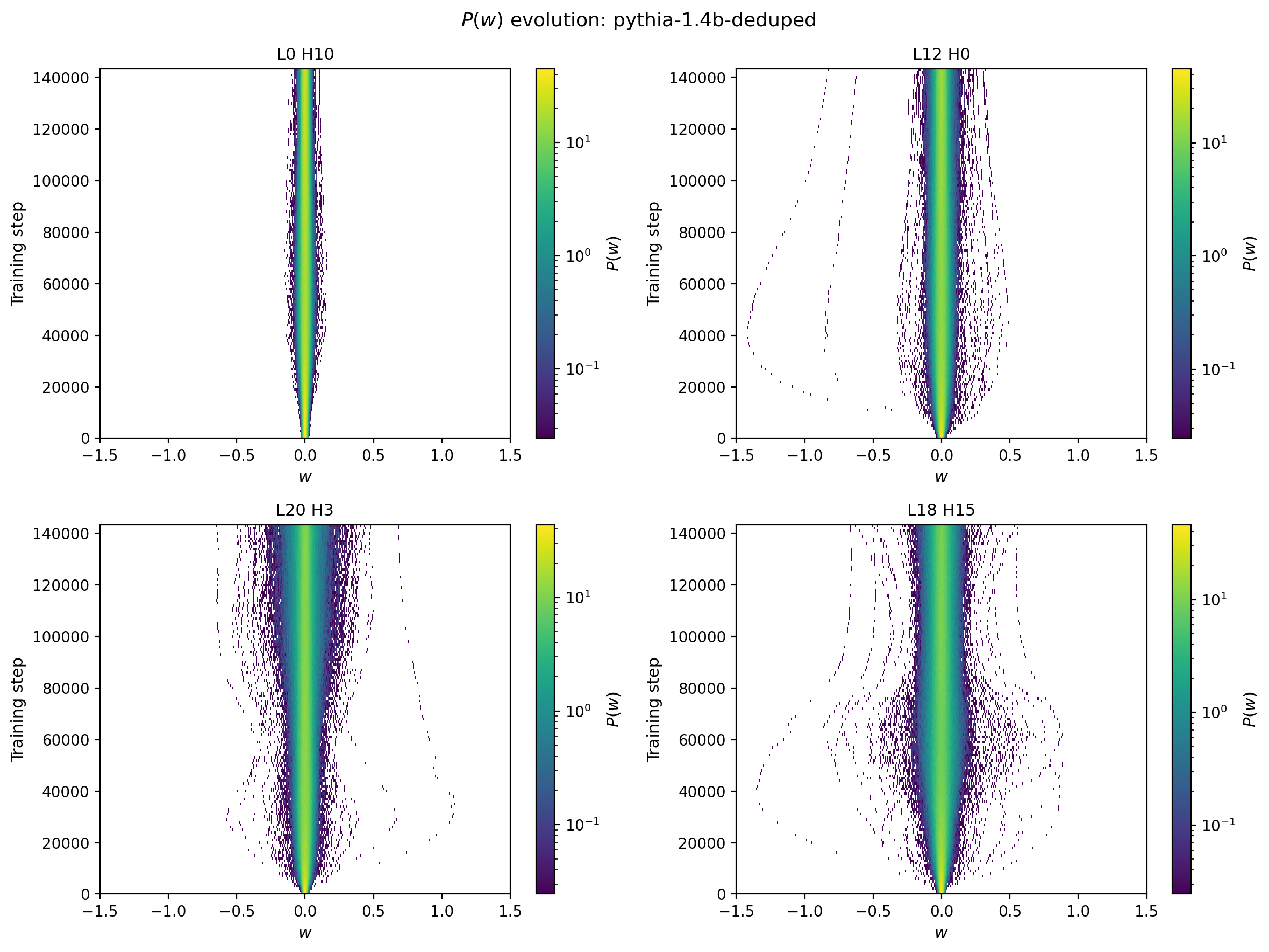
Figure 1: Element-wise probability distributions of $W_{QK}$ shown in 2D as a function of training step for four different attention heads.

It is noteworthy that changes in the time-evolution of $\sigma$ are generally accompanied by sharp jumps in the KL divergence. Furthermore, many of these transitions occur at different training steps for different heads. While some of the smooth global features in the evolution of these statistics may be driven by optimizer and scheduler choices, many of these time-localized transitions suggest abrupt changes in the model’s capacity.

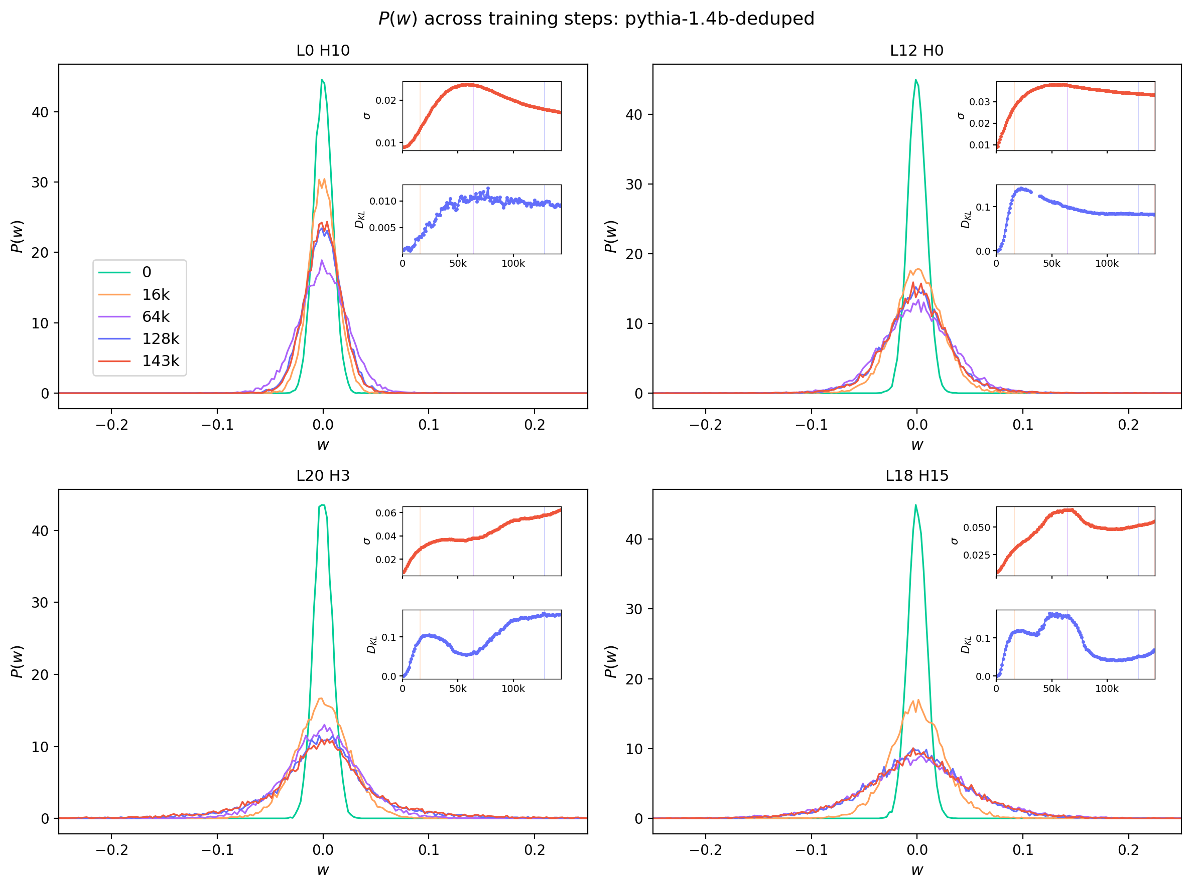
Figure 2: Element-wise probability distributions for $W_{QK}$ at selected training steps, shown for four different attention heads [TODO add layer x head numbers]. Shown in the insets are the full time dependence of the $\sigma$ and $D_{KL}(P(w) \,||\, N(\mu,\sigma))$ statistics, with the selected time slices indicated by vertical lines of matching color.

Head Diversity Within a Layer

The multi-panel view below highlights this within-layer diversity. Each panel overlays the time trajectories of all 16 heads in a single layer, with a layer-mean curve drawn in red dashed: the left panel tracks $\sigma$ and the right panel tracks $D_{KL}(P(w)||N(\mu,\sigma))$.

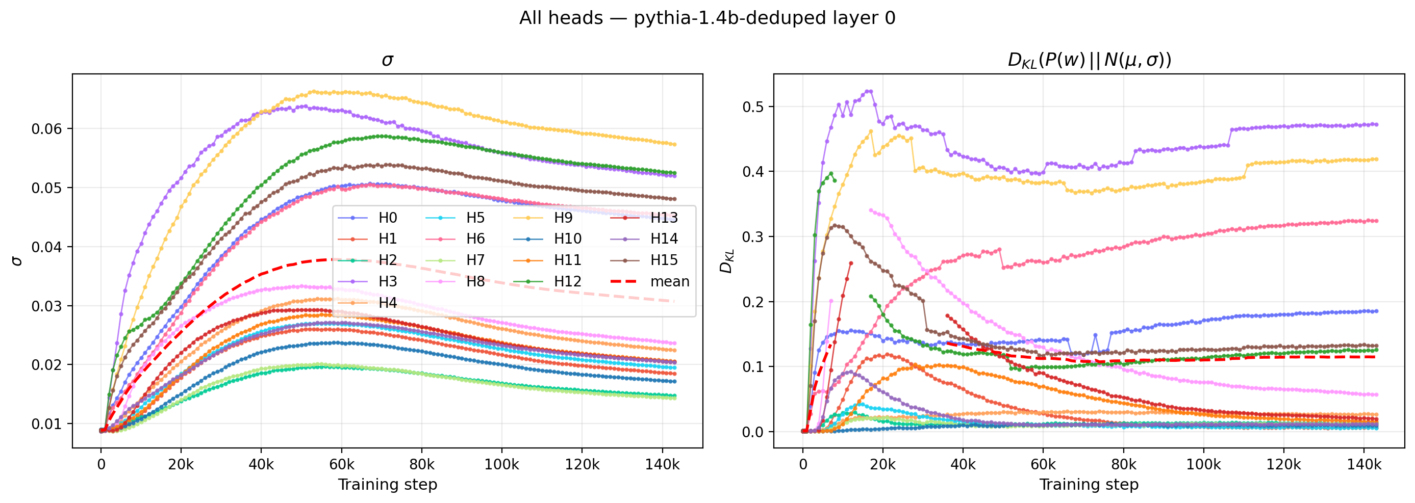
Figure 3: Time trajectories of $\sigma$ (left) and $D_{KL}(P(w)\,||\,N(\mu,\sigma))$ (right) for all 16 heads in a single layer of Pythia-1.4B. Heads within the same layer develop qualitatively different training dynamics.

Some heads rise monotonically to their final value; others exhibit non-monotone behavior with an early overshoot that partially relaxes. A few heads remain near their initialized values for a substantial fraction of training before rapidly converging. This heterogeneity within a single layer suggests that the dynamics of individual attention heads are not well-described by a single timescale or trajectory type.

Time Evolution Across All Heads

Using these statistics as a guide, we can examine the model behavior more comprehensively by comparing the time dependence across all layers and heads.

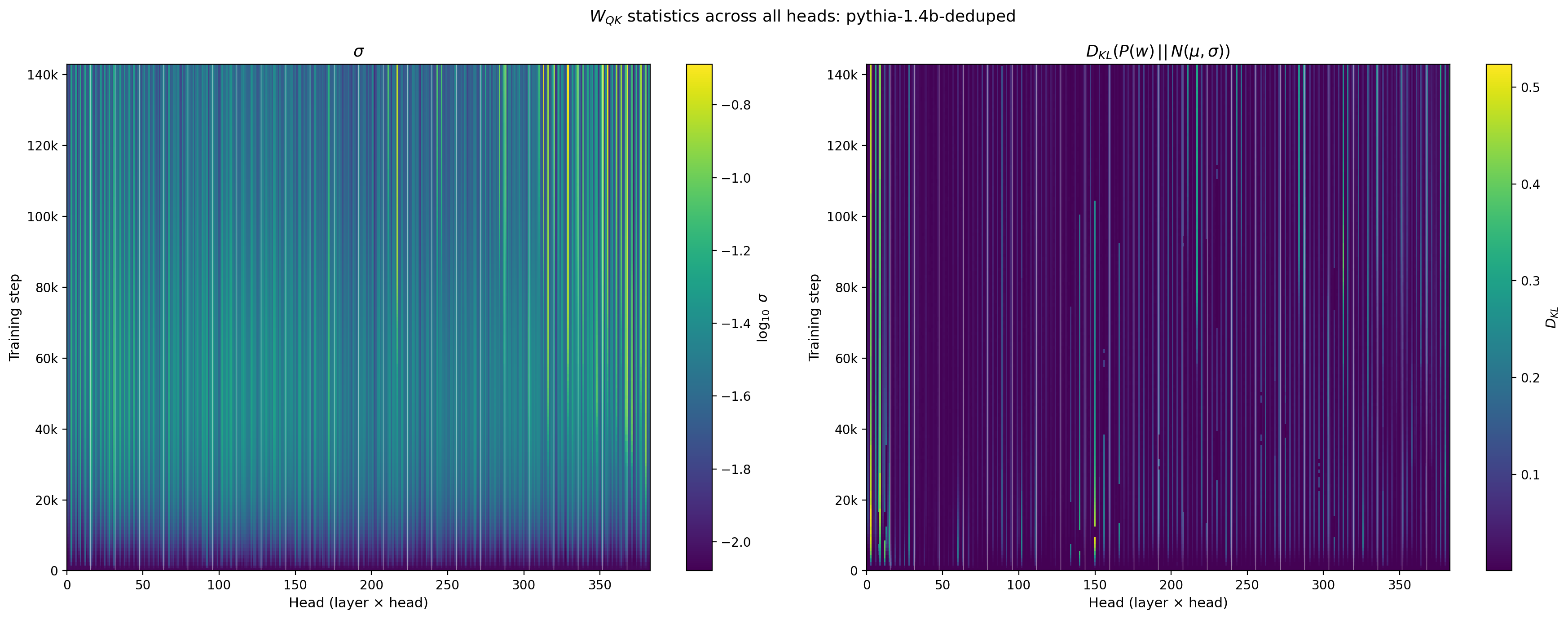
Figure 4: Standard deviation $\sigma$ (left, log color) and $D_{KL}(P(w)\,||\,N(\mu,\sigma))$ (right, linear color) of $W_{QK}$ across all 384 attention heads in Pythia-1.4B (16 heads × 24 layers), shown as a function of training step. White vertical lines mark layer boundaries.

Several features are apparent. The early-layer heads develop larger $\sigma$ values earlier. The within-layer spread — visible as variation within each layer block — increases over training and does not disappear: the heads within a layer diversify rather than converging toward a common value. This is consistent with the functional specialization hypothesis, in which heads within a layer develop distinct roles that are reflected in their weight statistics.

Time-Dependent Spectral Analysis

The spectral statistics from the singular value post can be tracked as a function of training step in exactly the same way as the element-wise statistics above. Figure 5 shows the SVD spectrum, displayed as eigenvalues $\lambda_k = \sigma_k^2$, for the same four reference heads as a function of singular-value index $k$ and training step. Almost immediately these heads become dominated by single leading singular values, while at still-early times the SVD spectrum rebalances and becomes flatter with larger singular values persisting at higher index. The distributions then narrow again but to different limiting behaviors.

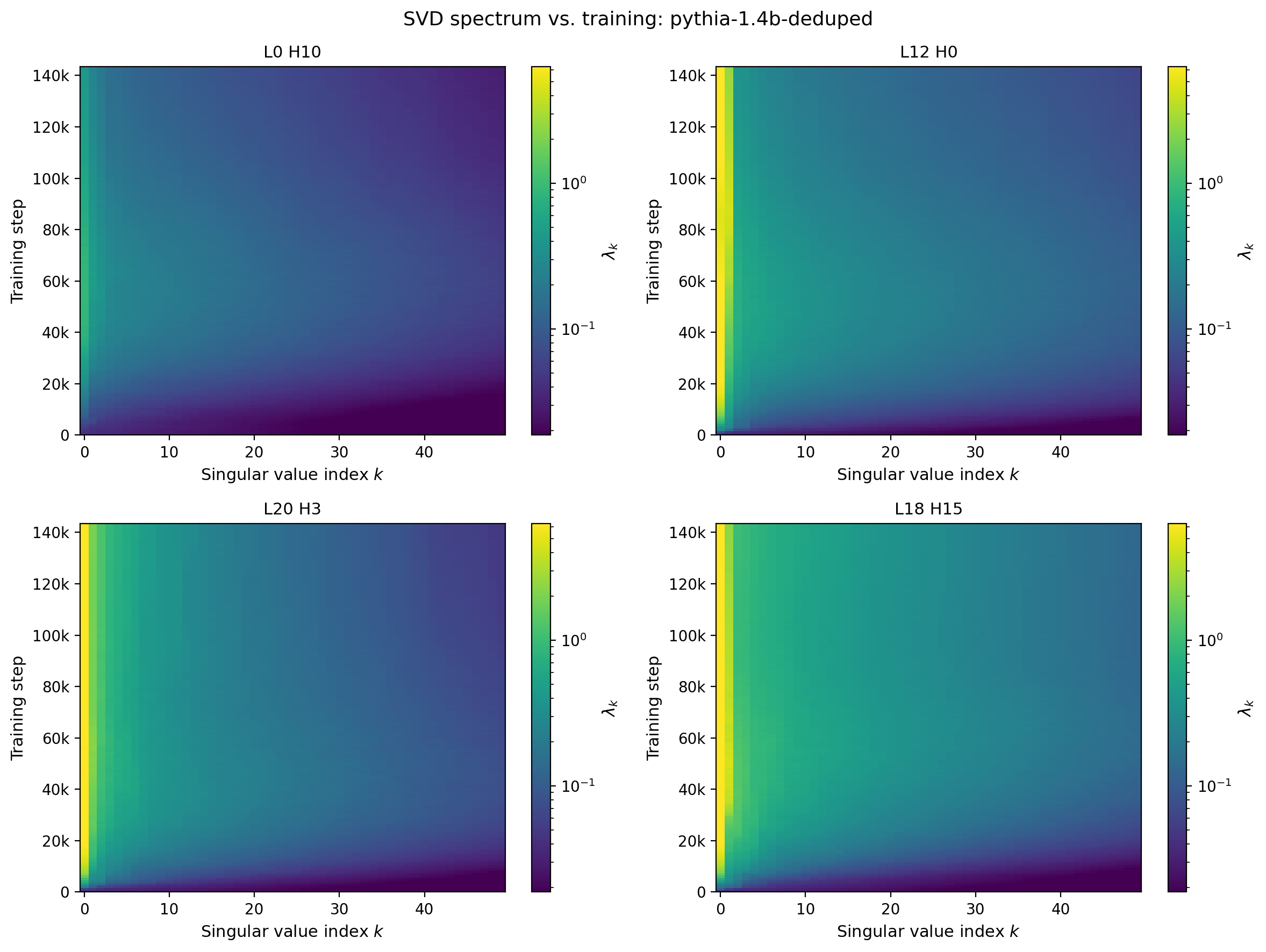
Figure 5: Squared singular values $\lambda_k = \sigma_k^2$ of $W_{QK}$ versus index $k$ and training step for four reference attention heads of Pythia-1.4B [TODO put in layer/head values used in the figure]. Color encodes $\lambda_k$ on a shared scale across panels.

The same evolution can be sliced at fixed steps to make the rearrangement of weight between leading and sub-leading singular values explicit. Figure 6 plots $\lambda_k$ versus $k$ at five training-step snapshots, in the same style as Figure 2.

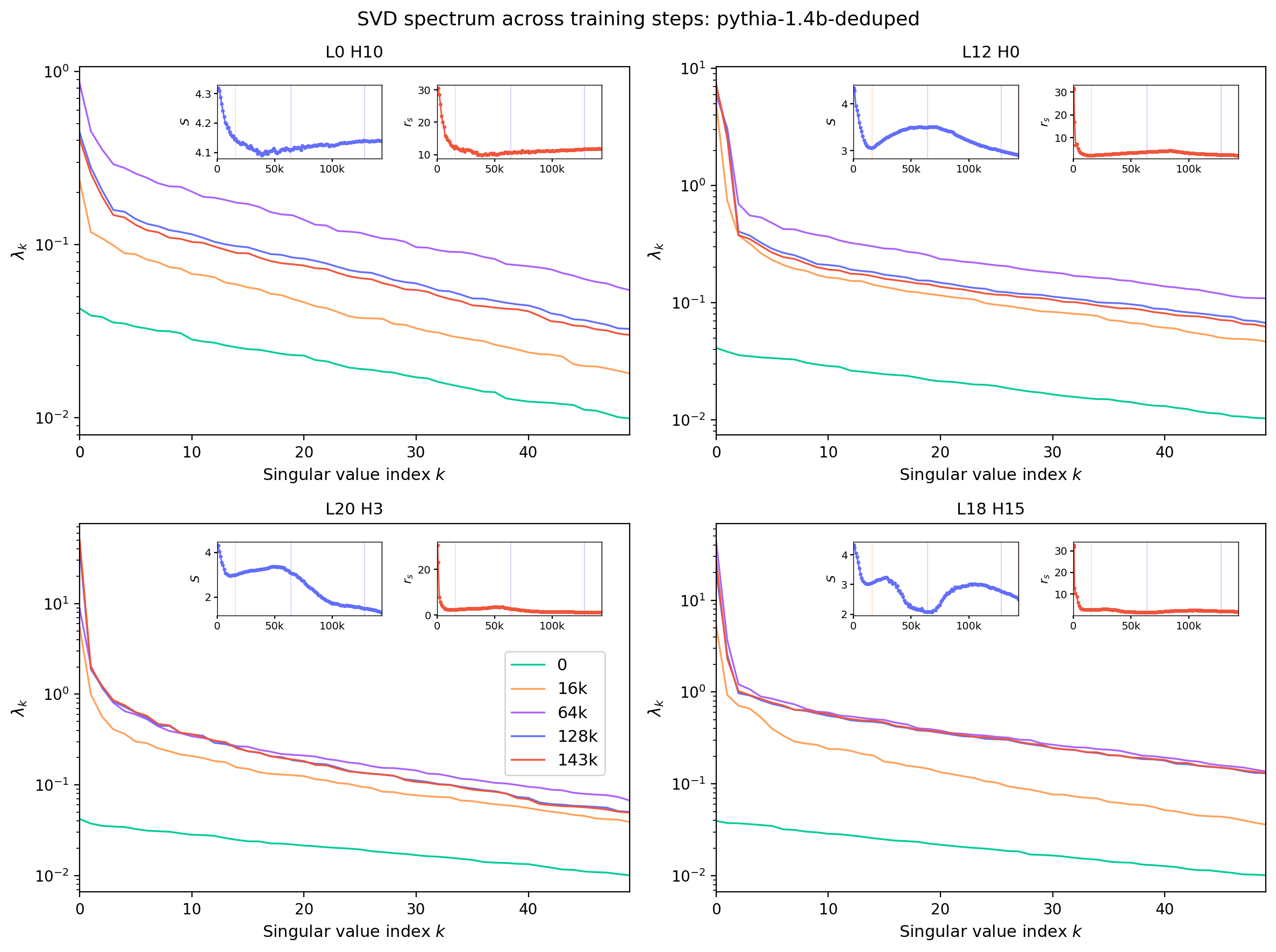
Figure 6: Squared singular values $\lambda_k$ versus index $k$ at five selected training steps for the same four reference heads as Fig. 5. Insets show the time evolution of two spectral summary statistics — the stable rank $r_s = \|W\|_F^2 / \|W\|_2^2$ and the spectral entropy — for the same head, with vertical lines marking the slice steps. These are discussed further in the next section.

This behavior is clearest when the time evolution of the leading eigenvalues themselves is shown directly. Figure 7 plots $\lambda_0,\ldots,\lambda_3$ as a function of training step for each reference head. The upper right panel (L12, H0) exhibits particularly interesting behavior. The leading eigenvalue reaches a maximum at $t\approx 30$k and begins to fall while the sub-leading eigenvalue continues to increase. As the two values approach one another the slope of the respectivel time-dependences flips sign. This could be an example of level repulsion in the training or level crossing, and can be further investigated by studying how the respective eigenvectors change: if the eigenvectors associated with each of the eignevalues remain roughly constant, this would correspond to repulsion, while if the leading and sub-leading eigenvectors swap, then the phenomenon is a level crossing. This timeslice roughly corresponds to infection points in the time dependence of the SVD-based statistics ($S$ and $r_{\text{S}}$).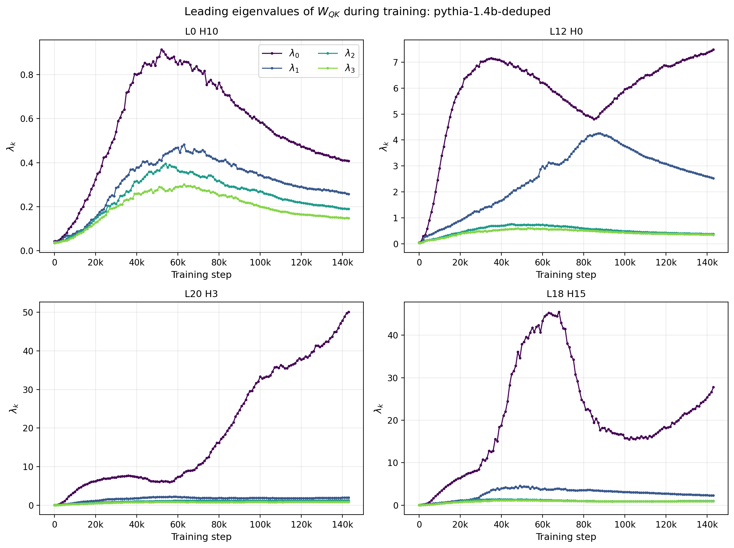

Figure 7: Trajectories of the four leading eigenvalues $\lambda_0,\ldots,\lambda_3$ of $W_{QK}$ as a function of training step for four reference attention heads of Pythia-1.4B. The relative gap between $\lambda_0$ and the sub-leading eigenvalues evolves non-monotonically in several heads.

For a deeper exploration of how individual eigenvalues evolve across all layers and heads — including the layer-averaged trajectory views — see Sections 8 and 9 of the interactive dashboard, which expose per-index trajectories with sliders for layer, head, and singular-value index.

Spectral Statistics

The same head-diversity and all-architecture views developed for $\sigma$ and $D_{KL}$ above can be repeated using spectral summary statistics. As noted in a previous post, statistics like the (normalized) particiption ratio correlate strongly with the spectral entropy, to provide more complementary information we introduce stable rank $r_s = |W|_F^2 / |W|_2^2$.

Both this quantity and the spectral entropy quantify how concentrated the spectrum is on a few leading directions but do so with different sensitivities to the tail. Note that both the normal distribution and MP distribution are from the same family of distributions with a known relationship between the entropy and the standard deviation: \(S(\sigma; q) \approx \log s^2 + g(q)\) where $q$ are some parameters of the distribution and $g(q)$ can be determined by calculation or direct numeric evaluation, but crucially, does not depend on $\sigma$. The utility of this feature is that when we empirically see similar relationships between the width and entropy in both the spatial and spectral domains, logarithmic growth with a distribution-dependent constant offset, we are probing complementary views of the deviation from Gaussianity. In the spatial case we quantified the deviation between the empirically determined sample entropy and the normal expectation by evaluating $D_{KL}(P(w)\,||\,N(\mu,\sigma))$, which is essentially the difference between these two entropies. The analogous statistic would be $D_{KL}(P(\lambda)\,||\,MP(\sigma, q=1/n_h))$, where $MP$ is the Marchenko-Pastur density. The normal and MP expectations are themselves approximations: as noted in previous posts, $W_QK$ is a product of random matrices and isn’t purely normally distributed nor do the eigenvalues obey a pure $MP$ distribution. We leave the task of a rigorously defining a random “null hypothesis” from the matrix ensembles for future and for now use the spectral entropy rather than the appropriate KL divergence. The time step dependence of these two quantities is shown in the insets of Fig. 6.

The time dependence for these two quantities for all heads within a given layer (L0) are shown in Fig. 8. Both quantities exhibit a sudden drop early in training although the slope and depth of this drop varies widely across heads. In most cases, the values reach their minima before 20k steps and begin a slow growth before flattening with very small slope. A few of the heads with large values of the stable rank turn over slighly at the latest times. In a few cases (e.g. H8), the slow growth does not occur and the different heads have different numbers of sign changes in their derivatives, resulting in qualitative differences in their time evolution. It should be noted that the “spatial” domain statistics do not depend on the matrix structure (statistics are computed from the distribution of matrix element s without reference to their position), while the spectral statistics explicitly involve the matrix structure, thus these two measures really do provide complementary information.

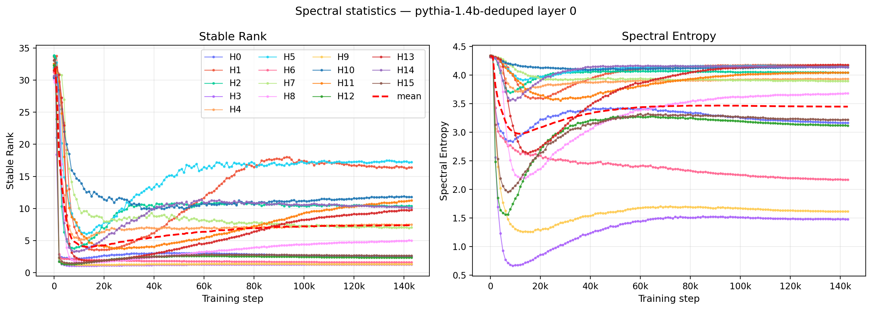
Figure 8: Time trajectories of the stable rank (left) and the spectral entropy (right) for all 16 heads in a single layer of Pythia-1.4B. The layer mean is overlaid as a red dashed curve.

Further generalizations are provided in Fig. 9, which shows the training trajectories for all layers and heads in the model for these same two statistics. While the features described above for the time-dependence hold for the majority of heads, the heatmaps show specific layer/head combinations where the behavior is qualitatively different.

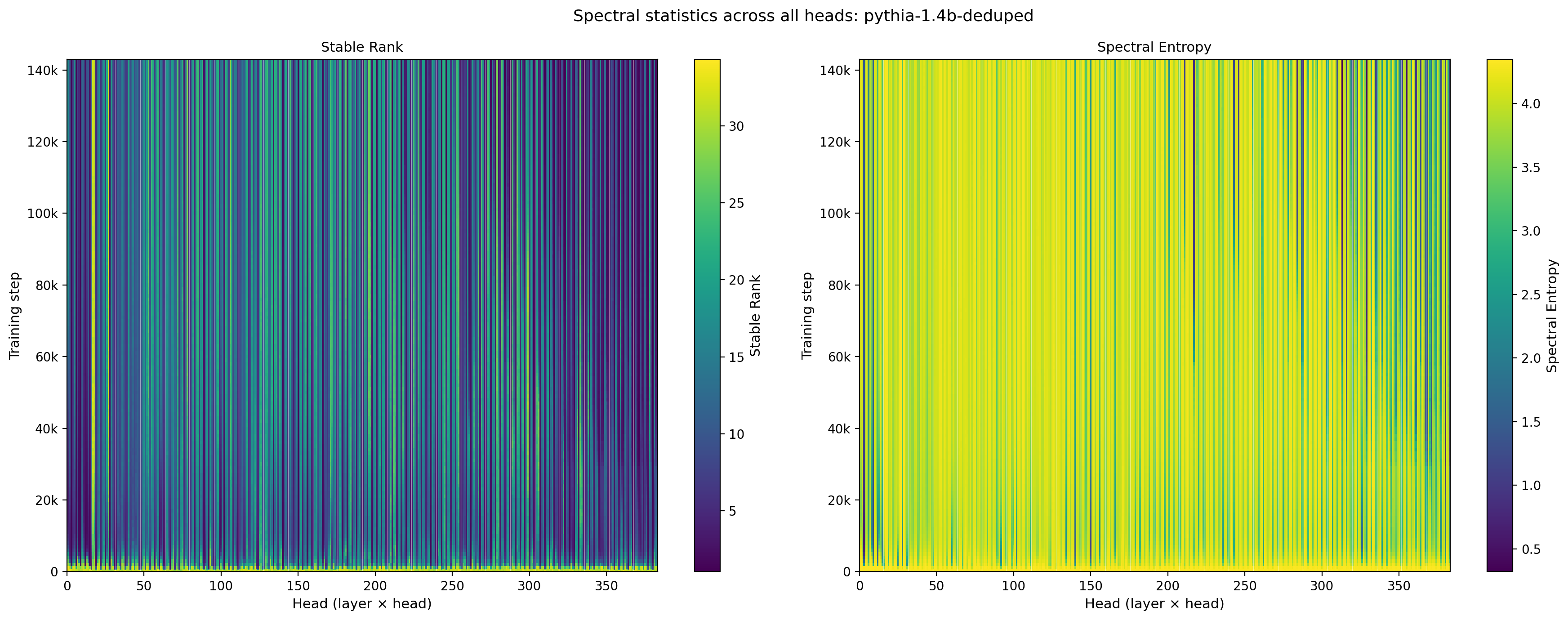
Figure 9: Stable rank (left) and spectral entropy (right) of $W_{QK}$ across all 384 attention heads in Pythia-1.4B, shown as a function of training step. White vertical lines mark layer boundaries.

As with the element-wise statistics, the spectral views show pronounced within-layer diversity and layer-dependent timing of the early-training transitions.

UMAP of Training Trajectories

To visualize the diversity of head trajectories more globally, we apply UMAP to the time series of head-level statistics, embedding each head’s full training trajectory as a point in two dimensions. Heads whose trajectories evolve in similar ways appear nearby in this embedding. We show the embeddings for two complementary statistics $D_{KL}(P(w)\,||\,N(\mu,\sigma))$ and the spectral entropy, which are complementatry as the operate in the spatial and spectral domains respectively.

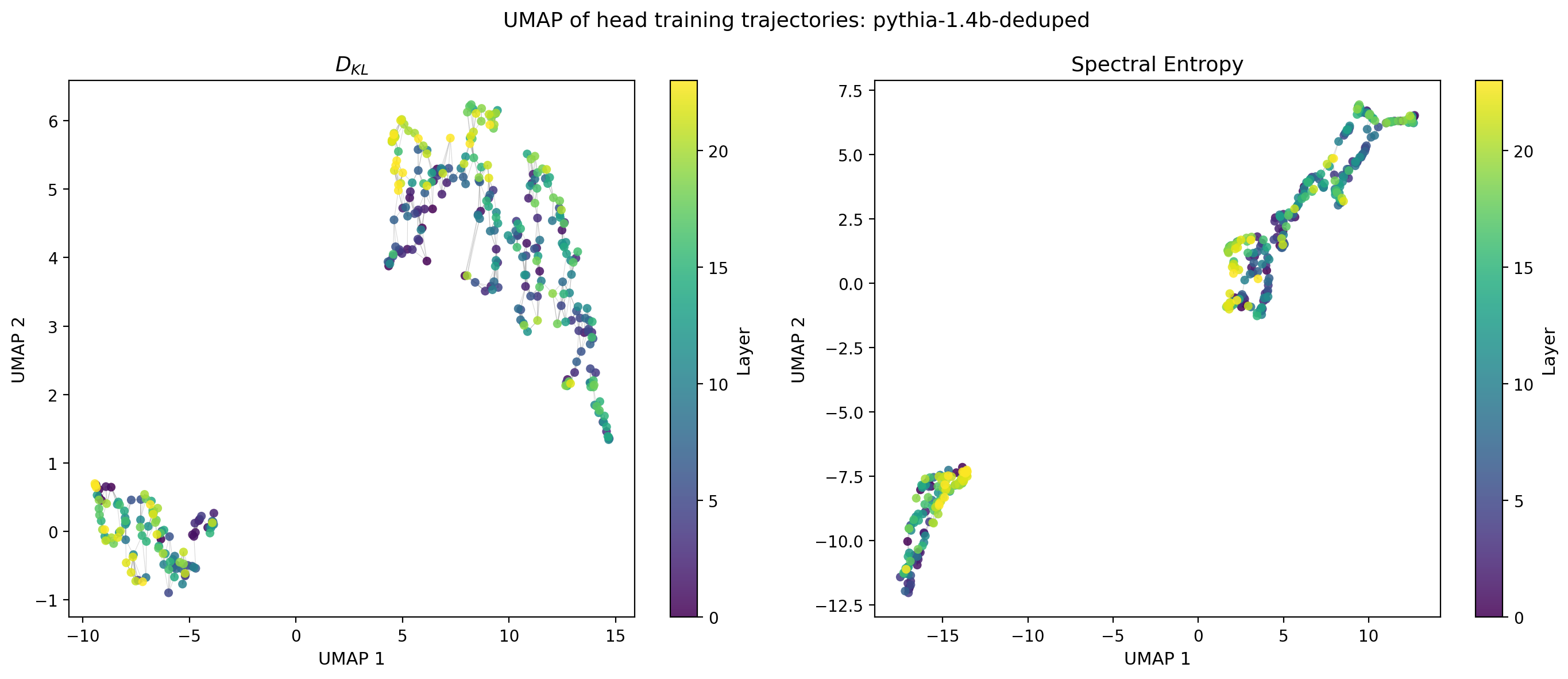
Figure 10: UMAP embeddings of training-step trajectories of $D_{KL}(P(w)\,||\,N(\mu,\sigma))$ (left) and the spectral entropy (right) for all attention heads in Pythia-1.4B. Points are colored by layer; gray edges show the $k$-nearest-neighbour graph in UMAP coordinates.

The embeddings reveal a two qualitatively distinct trajectory types. The element-wise and spectral views show similar overall organization, suggesting that the same trajectory taxonomy is visible regardless of which summary statistic is used. Whether these clusters correspond to functional head types, or different types of “learners” is a natural question for future work.

Interactive Animations

The static heatmaps in Figs. 4 and 9 collapse the time axis into a second spatial dimension; an alternative is to keep the layer × head architecture as the primary view and step through training time directly. The two embeds below provide that view for $\sigma$ and the stable rank: the central panel shows the statistic across all 384 attention heads of Pythia-1.4B at a fixed step, with marginal traces showing the head-averaged trajectory by layer (right) and the layer-averaged trajectory by head (bottom). Use the play button or scrub the slider to advance through the 154 checkpoints.

Figure 11: Architecture-wide evolution of $\sigma$ across training. The central heatmap shows $\sigma$ for every (layer, head) at the selected training step; right and bottom marginals are the layer- and head-averaged values at that step.

Figure 12: Architecture-wide evolution of the stable rank $r_s = \|W\|_F^2 / \|W\|_2^2$ across training, in the same format as Fig. 11.

Played end to end, the early-training rearrangement that drives the heatmaps in Figs. 4 and 9 is immediately visible: the $\sigma$ animation shows the within-layer spread widening through the first ~20k steps before settling into a slowly-drifting steady state, while the stable-rank animation makes the rapid early collapse onto a few leading directions, and the subsequent partial recovery, easier to follow than any static slice.

What Comes Next

The analyses here use Pythia-1.4B as a reference, but the checkpoint data covers the full Pythia suite. A natural extension is to ask whether the trajectory types identified here — the timescales, the UMAP cluster structure, the pattern of early-layer consolidation — are universal across model scales or change systematically with parameter count. The Pythia suite, with its consistent training setup across scales, provides a controlled setting for that comparison.

The code, data, and interactive dashboards for reproducing and extending this analysis are available at the links above.