Inverse Scattering via Physics-Informed Neural Networks
Published:
Spectral Structure in Neural Network Solutions of the KdV Equation
Introduction
In this post I train a physics-informed neural network (PINN) to learn the behavior of soliton solutions to the Korteweg–de Vries (KdV) equation in 1+1 dimensions. PINNs are trained using loss functions derived from the equations of motion and the boundary conditions of the physical problem. Unlike traditional numerical solvers, these networks are inherently differentiable, a property that is directly accessible through automatic differentiation in frameworks like PyTorch.
The KdV equation is a classic example of an integrable system: it admits an infinite set of conservation laws, each constraining the field dynamics locally at every spacetime point. I use these conservation relations as independent, unsupervised diagnostics. The procedure enables you to generate an arbitrary number of loss measures that quantify exactly how well the PINN represents the underlying physics, without feeding directly into the training objective. The tradeoff is that these terms involve increasingly higher-order derivatives, which can lead to numerical instability and large computational graphs, although the automatic differentiation tools available in modern machine learning frameworks offer several strategies to manage this.
This integrability property has deep mathematical foundations that connect many ideas across mathematics and physics. The inverse scattering framework has found applications across these domains, and it provides a useful setting for studying how learned solutions inherit structural properties. I focus here on the Inverse Scattering Transform (IST), which reframes the initial-boundary value problem in a way that is particularly well-suited to the PINN setting.
Where a conventional boundary value problem specifies $u(x,t)$ or its normal derivative at the domain boundary (Dirichlet vs Neumann), the IST formulation specifies instead the scattering data, associated with a Schrödinger operator $L = -\partial_x^2 - u$. The problem of reconstructing $u$ from this data is a Riemann-Hilbert problem. Because $L$ has the structure of a quantum mechanical Hamiltonian the scattering data, $\mathcal{S} = {R(k); (\kappa_n, c_n)}$, specifies information about bound states and scattering states.
This enables a complementary test: I extract the eigenvalues and eigenstates from the learned potential and check whether the PINN solution preserves the spectral properties (isospectrality and the correct eigenfunction dynamics) that characterize exact solutions. The results demonstrate that basic PINN formulations can capture the full spectral structure of an integrable system, providing an example of how deep mathematical properties of exact solutions transfer to the learned model without explicit inductive bias.
The IST program can be viewed as a non-linear method of images, where instead of introducing image charges to match boundary conditions the IST state object describes the local density of image charges. This provides a powerful tool for specifying boundary conditions as real-world constraints are often better suited to this description. It also provides an interpretable state representation that provides a natural framework to introduce bias, feedback, measurement and uncertainty.
Background
The KdV Equation and Inverse Scattering
The KdV equation is a nonlinear dispersive wave equation, \(u_t + 6uu_x + u_{xxx} = 0\)
The nonlinear term $6uu_x$ represents velocity-dependent advection: regions of larger amplitude propagate faster, steepening the wave profile. The dispersive term $u_{xxx}$ counteracts this steepening by spreading different frequency components at different speeds. The soliton arises from the exact balance between these two effects, originally observed in the context of shallow water waves where the KdV equation describes the evolution of long-wavelength surface disturbances in a channel of finite depth.
The single-soliton solution, selected by requiring the wave to vanish at spatial infinity, is
\[u = 2\kappa^2 \operatorname{sech}^2[\kappa(x - 4\kappa^2 t - x_0)]\]where $\kappa$ determines both the amplitude ($2\kappa^2$) and the velocity ($4\kappa^2$): taller solitons travel faster. As noted above, the KdV equation admits an infinite set of conserved quantities $(\rho_i[u], J_i[u])$ satisfying $\partial_t \rho_i + \partial_x J_i = 0$. The first several are shown in Table 1.
| Quantity | $\rho_i$ | $J_i$ |
|---|---|---|
| Mass ($i=0$) | $u$ | $3u^2 + u_{xx}$ |
| Momentum ($i=1$) | $\frac{1}{2}u^2$ | $2u^3 + uu_{xx} - \frac{1}{2}u_x^2$ |
| Energy ($i=2$) | $-u^3 + \frac{1}{2}u_x^2$ | $-\frac{9}{2}u^4 - 3u^2 u_{xx} + 6u u_x^2 + u_x u_{xxx} - \frac{1}{2}u_{xx}^2$ |
Table 1: Conserved densities and fluxes for the KdV system. Each pair satisfies $\partial_t \rho_i + \partial_x J_i = 0$ independently.
The Lax representation reformulates the KdV equation as the compatibility condition for a pair of linear operators $(L, A)$:
\[L_t = [A, L]\]where
\[L = -\partial_x^2 - u\,,\quad A = -4 \partial_x^3 - 6u\partial_x - 3u_x\]The operator $L$ is a Schrödinger operator: it has the form of the Hamiltonian from nonrelativistic quantum mechanics with $u$ playing the role of the potential. This suggests a complementary formulation in terms of the eigenstates of $L$,
\[L\psi_n = \lambda_n \psi_n\]for which the Lax equation implies
\[\frac{\mathrm{d}\lambda_n}{\mathrm{d}t} = 0\,,\quad \frac{\partial \psi_n}{\partial t} = A \psi_n\]The eigenvalues are independent of time (the isospectral property) and $A$ is a time-evolution operator for the eigenstates. This means that instead of solving the KdV equation for $u(x,t)$ subject to initial and boundary conditions on $u$, one can specify conditions on the scattering states and reconstruct $u$ from the spectral data. This is the inverse scattering transform (IST).
For reflectionless $N$-soliton solutions, the scattering data consists of the discrete eigenvalues $\lambda_n = -\kappa_n^2$ and norming constants $c_n(0)$. The solution is reconstructed as
\[u^{\text{IST}}(x,t) = 2\partial_x^2 \log \det M\]where the matrix $M$ is constructed from the scattering data:
\[M_{mn} = \delta_{mn} + \frac{c_m\, c_n\, e^{(\kappa_m + \kappa_n)x}}{\kappa_m + \kappa_n}\,,\quad c_n(t) = c_n(0)\, e^{-4\kappa_n^3 t}\]Further details on the $\tau$-function formulation used for numerical stability appear in the Appendix.
 Movie 1 A single soliton (black) with $\kappa$ = 2 and corresponding eigenstate (purple), which remains trapped in the potential produced by the solition.
 Movie 2 An eight soliton train, intially ordered from largest to smallest $\kappa$ value, so that the fastest solitons overtake the slower ones in a cascading effect. The solitons are reflectionless and gradually separate, returning to their original shapes.
Physics-Informed Neural Networks
A physics-informed neural network approximates the solution to a PDE by training a neural network $u_\theta(x,t)$ whose loss function encodes the governing equations. For the KdV equation, the loss takes the form
\[\mathcal{L} = \lambda_{\text{PDE}}\,\mathcal{L}_{\text{PDE}} + \lambda_{\text{SD}}\,\mathcal{L}_{\text{SD}}\]where the PDE loss, $\lVert u_t + 6uu_x + u_{xxx} \rVert_{2}^{2}$, is evaluated at collocation points in the domain interior, and $\mathcal{L}_{\text{SD}}$ encodes the scattering data $\mathcal{S}$ at the domain boundary.
The key feature distinguishing PINNs from standard regression is that the PDE residual involves derivatives of the network output with respect to its inputs. These are computed exactly using automatic differentiation, the same backpropagation machinery used for gradient descent, rather than finite differences.
Minimizing the PDE residual drives the network toward a function that satisfies the differential equation pointwise. However, a small PDE residual does not by itself guarantee that the solution is physically correct; it only ensures that $u_t + 6uu_x + u_{xxx} \approx 0$ at the sampled collocation points. Whether the learned solution also respects the deeper structural properties of the equation (conservation laws, integrability, spectral structure) is a separate question, and the one this post seeks to address.
Analytical Tooling
Before building the PINN, I developed several analytical and computational tools that serve both to validate the implementation and to provide independent diagnostics for the learned solutions.
The first component is an IST solver that constructs exact $N$-soliton solutions from the scattering data ${\kappa_n, c_n(0)}$. The matrix $M$ is built as a differentiable tensor, preserving its dependence on the input coordinates so that $u = 2\partial_x^2 \log \det M$ can be evaluated exactly via autograd. This was cross-checked against an independent implementation using the $\tau$-function formulation with analytically computed derivatives. The solver also provides the corresponding eigenstates $\psi_n(x,t)$ from the same scattering data.
A second component solves the Schrödinger eigenvalue problem $L\psi = \lambda\psi$ at each time slice using finite-difference discretization of $L = -\partial_x^2 - u$. This accepts an arbitrary potential $u$, whether from the IST solver or from the neural network, and returns the eigenvalues and eigenfunctions. The key diagnostic is whether the eigenvalues remain constant in time (isospectrality) and whether the eigenfunctions exhibit the correct exponential time dependence.
The third component evaluates the full KdV conservation hierarchy, computing the densities $\rho_n$, fluxes $J_n$, and local residuals $\partial_t \rho_n + \partial_x J_n$ for any input field via autograd. All three components operate on the same tensor representation, so they can be applied interchangeably to exact and learned solutions, enabling direct comparison.
Figure 1 shows the analytic 2-soliton solution and its derivatives, computed from scattering data with $\kappa = (1.5, 1.4)$ and initial positions chosen so the solitons are well-separated throughout the domain. The two solitons travel at slightly different speeds ($v = 4\kappa^2$), producing nearly parallel trajectories. The conservation law residuals for this solution are shown in Figure 2, confirming that all three hierarchy relations vanish to numerical precision across the domain.
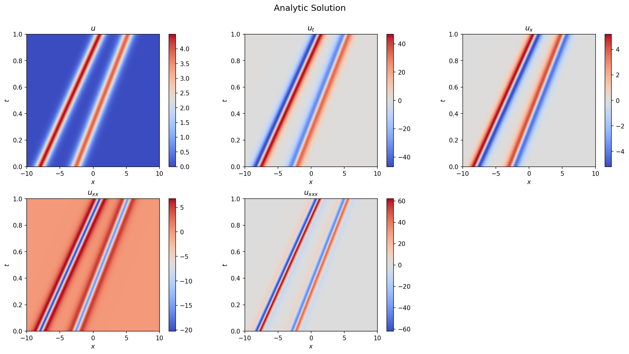 Figure 1: Spacetime field $u(x,t)$ and its derivatives for the analytic 2-soliton solution with $\kappa_1 = 1.5$, $\kappa_2 = 1.4$.
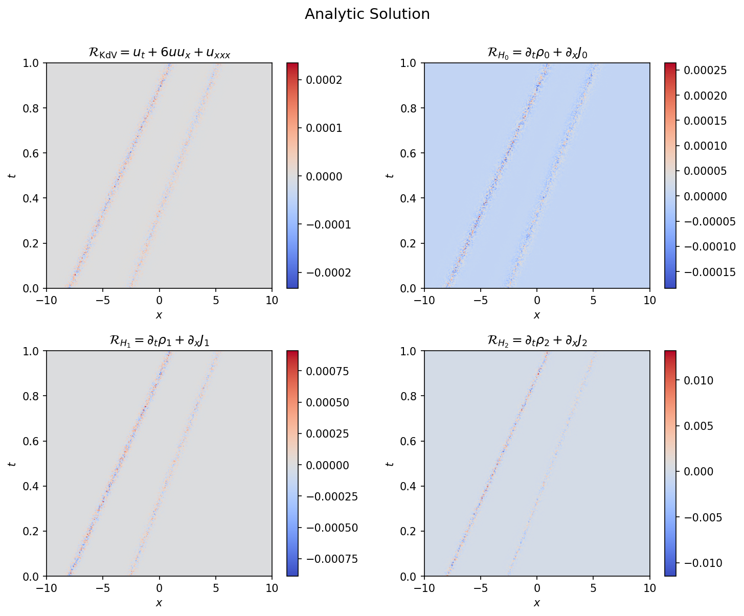 Figure 2: Conservation law residuals $\partial_t \rho_i + \partial_x J_i$ for the analytic solution. The KdV and mass conservation residuals are $\mathcal{O}(10^{-5})$; the higher-order energy residual reaches $\mathcal{O}(10^{-3})$, reflecting the accumulation of numerical error in the higher-order autograd chains. These residuals confirm the implementation of the IST solver and set the baseline for evaluating the PINN.
Neural Network Training
Architecture and Setup
The neural network is a multilayer perceptron with three hidden layers of 128 units each and $\tanh$ activation functions. The choice of $\tanh$ is motivated by the expected solution profiles: the $\operatorname{sech}^2$ shape of KdV solitons is the derivative of $\tanh$, so the activation functions are naturally suited to represent the sharp curvature at soliton boundaries.
The PDE residual and conservation laws are evaluated on a spacetime domain $(x,t) \in [-L, L] \times [0, T]$. Collocation points are generated using stratified sampling on an $N \times N$ grid with random jitter applied at each epoch to prevent the network from overfitting to specific grid locations. Boundary conditions are derived from the exact scattering data evaluated on the domain boundary, with the domain chosen so that all solitons have negligible support at $x = \pm L$ over $[0, T]$. The optimizer is AdamW with a learning rate of $10^{-3}$ and cosine annealing.
Pretraining
The optimization landscape is characterized by distinct topological sectors, each associated with a particular soliton configuration: the number of solitons, their ordering, and their relative phases. Gradient-based optimization initialized from a random network has no mechanism to select among these sectors, so it is important to initialize the model in the right basin of attraction.
To achieve this, the model is first pretrained using a supervised loss that compares directly to the analytic solution: \(\mathcal{L}_{\text{S}} = \| u_\theta(x,t) - u^{\text{IST}}(x,t;\mathcal{S}) \|_{2}^{2}\)
This loss is evaluated on the bulk interior points. As Figure 3 shows, the pretrained model does a good job of obtaining pointwise accuracy for $u$, capturing the complicated multi-soliton interaction structure. But it does so in a manner that neglects the field dynamics: the conservation law residuals are $\mathcal{O}(1)$ for the KdV equation and exceed 100 for the energy conservation relation, compared to $\mathcal{O}(10^{-5})$ for the analytic solution. The pretrained model has learned to interpolate the field values without learning the underlying dynamics.
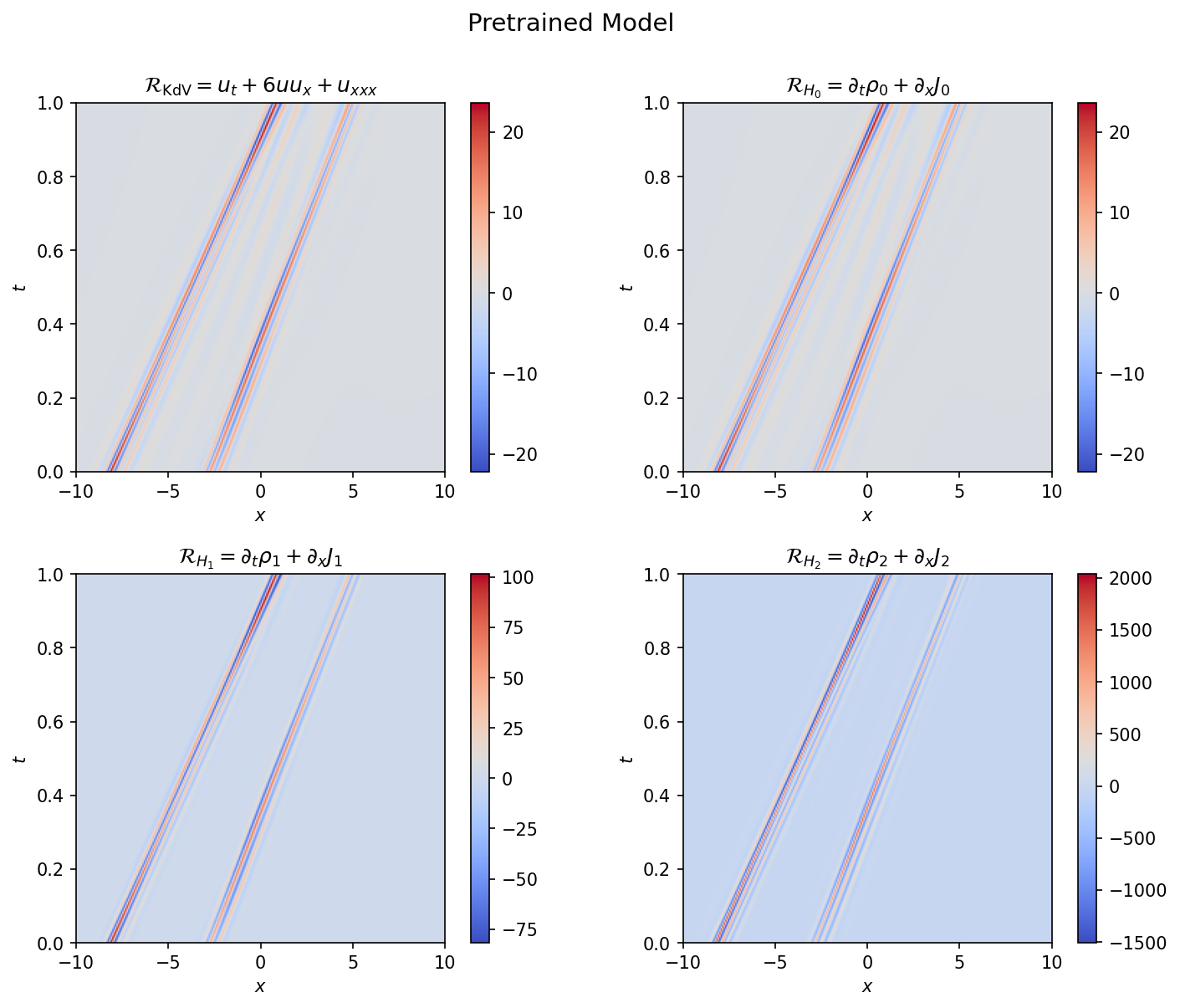 Figure 3: Conservation law residuals for the pretrained model. The residuals are $\mathcal{O}(1)$ for the KdV equation and exceed 100 for the energy conservation relation, localized along the soliton trajectories.
PINN Training
The PINN training replaces the bulk supervised loss with the KdV PDE residual, while retaining scattering-data-derived losses on the initial and boundary surfaces:
\[\mathcal{L} = \lambda_{\text{PDE}} \| u_t + 6uu_x + u_{xxx} \|_{2}^{2} + \lambda_{\text{SD}} \left( \mathcal{L}_{\text{S}} \Big|_{\text{IC}} + \mathcal{L}_{\text{S}} \Big|_{\text{BC}} \right)\]where the $\lambda$’s are hyperparameters controlling the relative weight of each term. The supervised loss $\mathcal{L}_{\text{S}}$ against $u^{\text{IST}}$ is also tracked over the bulk as a diagnostic but does not contribute to the training objective.
Early in training, the loss is dominated by the KdV residual. This is expected given the large derivative errors inherited from pretraining. If these residuals are so large the resulting updates can completely wipe out the pretrained field shapes, forcing the training to explore the full landscape instead of the topological sector selected by the pretraining. This can occur when the number of epochs used in the pretraining is large and the point estimates learned by the model are too sharp. Successful training runs allow the field dynamics to evolve through the KdV residual loss while maintaining the boundary conditions.
In practice the boundary conditions at spatial infinity decouple quickly, while the initial condition loss prevents zero mode collapse. The model struggles to learn configurations where the solitons have large overlap at $t=0$, or equivalently where the initial conditions are not specified at a time when the solitons are well separated. In these cases the optimization becomes confused among the different topological sectors.
Figure 4 shows the PINN training summary: loss curves (left) and the resulting spacetime field (right). The PDE loss dominates initially as the network corrects its derivative structure, then decreases steadily while the boundary losses remain small throughout. The supervised loss $\mathcal{L}_S$, which is tracked but does not contribute to the training objective, provides an independent measure of solution quality.
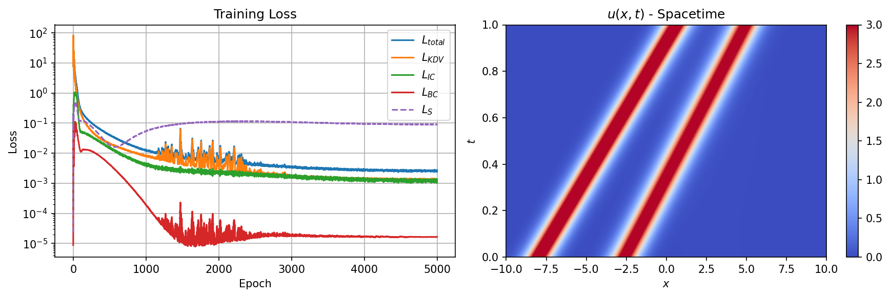 Figure 4: PINN training summary. Left: loss curves showing the PDE residual (blue), initial condition (orange), boundary condition (green), and tracked supervised loss (dashed). Right: learned spacetime field $u(x,t)$ after PINN training.
Also shown are the KdV hierarchy residuals (Figures 5 and 6). None of the conservation laws feeds directly into the loss except the zeroth-order relation, which reduces to the KdV equation. Note that even though analytically $\partial_t \rho_0 + \partial_x J_0 = 0$ reduces to the KdV equation, the numerics of evaluating this residual are slightly different since the autograd graph is constructed differently. The KdV and mass conservation residuals are $\mathcal{O}(10^{-1})$, substantially reduced from the pretrained model, with the largest values concentrated near the soliton interaction region. The higher-order energy residual is larger but still modest relative to the field amplitude. The results indicate that not only are the various integrals of motion preserved, the conservation relation holds well locally for all points in the domain, suggesting that the PINN training process has endowed the learned model with the KdV’s integrability properties.
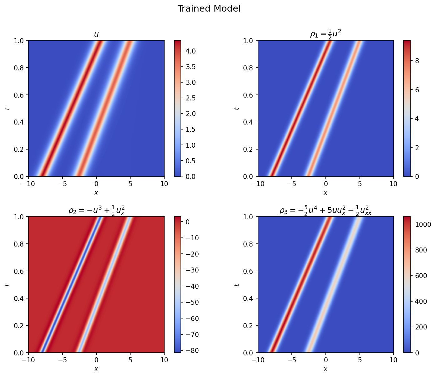 Figure 5: Conserved densities for the trained PINN: the field $u$, momentum density $\rho_1 = \frac{1}{2}u^2$, energy density $\rho_2 = -u^3 + \frac{1}{2}u_x^2$, and third-order density $\rho_3$.
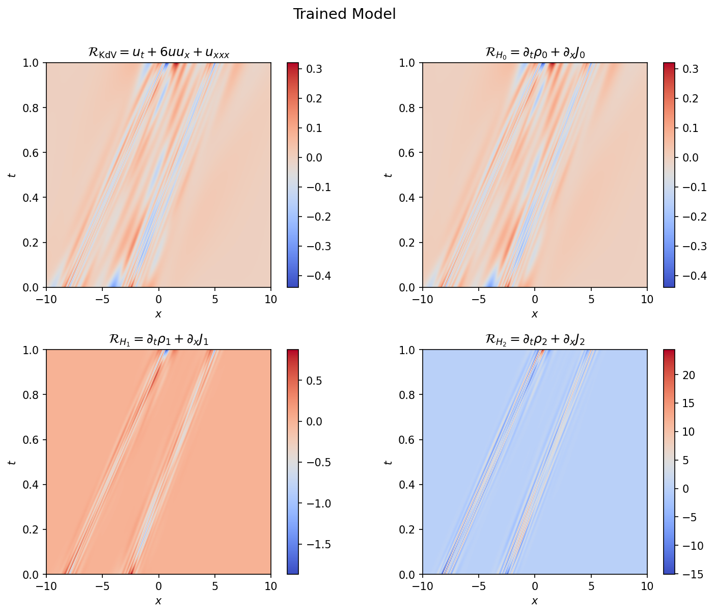 Figure 6: Conservation law residuals for the trained model. The KdV residual and mass conservation residual (left, center) are $\mathcal{O}(10^{-1})$, while the energy conservation residual (right) is larger. Only the KdV equation enters the training loss; the higher-order residuals serve as independent diagnostics.
Spectral Analysis of Learned Solutions
To test whether the PINN solution preserves the spectral structure of the KdV equation, I extract the eigenvalues and eigenstates from the Schrödinger operator $L = -\partial_x^2 - u$ constructed from the learned field $u(x,t)$. The eigenvalue problem is solved independently at each time slice using finite-difference discretization. For this analysis I switch to a more interesting configuration with $\kappa = (2.0, 1.5)$ where the solitons cross within the time domain.
Figure 7 shows the extracted eigenfunctions $|\psi_n(x,t)|^2$. Each eigenfunction is localized within the potential well created by its corresponding soliton and travels with that well. As the solitons travel at different speeds (different $\kappa$) they can overtake one another. When this occurs the eigenstates become delocalized to accommodate the wider effective potential. During this interaction, each eigenfunction develops a component that is out of phase with the original localized profile. This component grows until the slower soliton has transferred its amplitude behind the faster one, at which point the eigenfunction relocalizes, having acquired a phase shift.
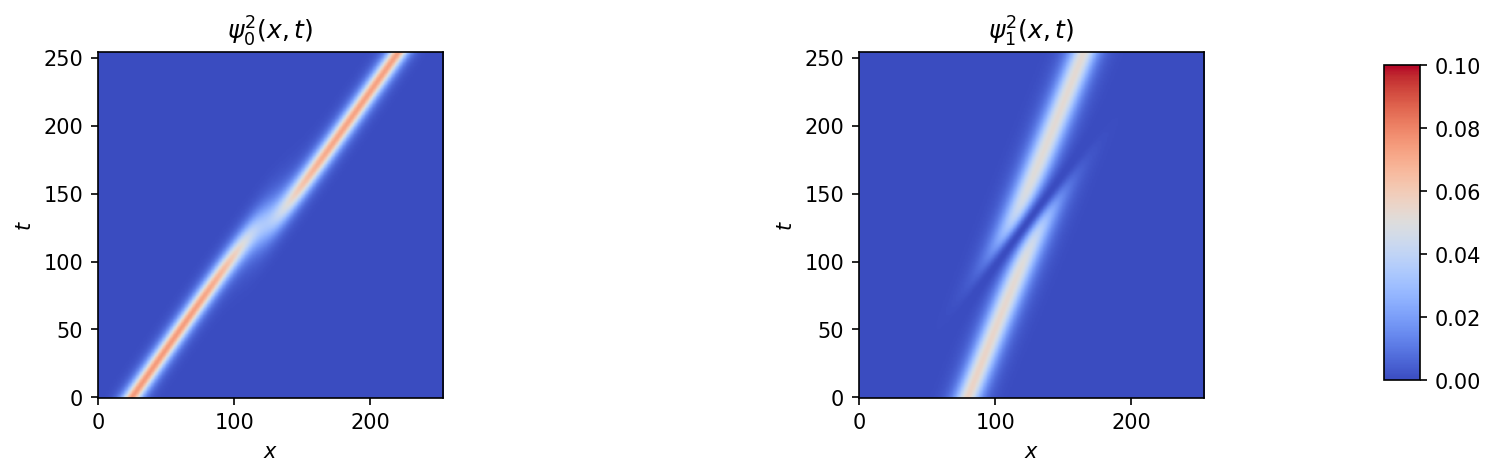 Figure 7: Squared eigenfunctions $|\psi_n(x,t)|^2$ extracted from the PINN-learned potential for the crossing 2-soliton configuration ($\kappa = 2.0, 1.5$). The eigenstates track the soliton trajectories and exhibit delocalization during the interaction region.
Figure 8 shows the recovered eigenvalues $\kappa_n = \sqrt{-\lambda_n}$ as a function of time, compared to the ground truth values specified as part of the scattering data. The eigenvalues agree well with the input values and remain approximately constant in time, exhibiting the isospectral property, although the eigenvalues have a net displacement from their ground truth values. This behavior occurs when the PINN solutions form well form solitons that evolve properly with time, but with the wrong slope in the $x-t$ plane. This pattern is observable in the training dynamics, when the PINN attempts to learn to increase the slope of a particular soliton but is prohibited by another nearby soliton. The PINN’s limitations in distingushing the two solitons in the spatial domain affect degredation of its spectral representation, but while generally preserving isospectrality: solutions look like propagating solitons for most times.
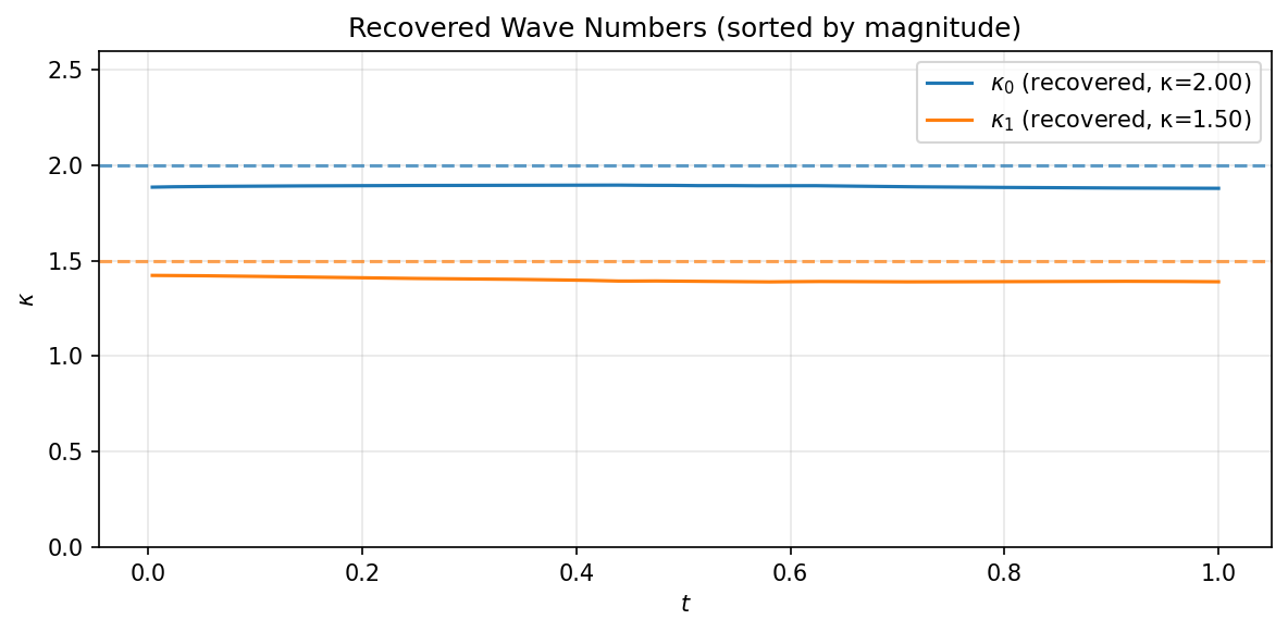 Figure 8: Recovered wave numbers $\kappa_n(t)$ for the crossing configuration (solid lines) compared to ground truth values (dashed lines). The approximate time-independence confirms the isospectral property.
Three-Soliton Results
To test whether these results extend to higher soliton number, I trained a PINN on a 3-soliton configuration with $\kappa = (2.0, 1.6, 1.4)$. The increased number of solitons produces a richer interaction structure with multiple pairwise collisions at different spacetime locations.
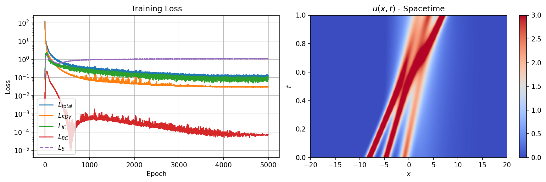 Figure 9: Training summary for the 3-soliton configuration. Left: loss curves. Right: learned spacetime field $u(x,t)$ showing the three soliton trajectories and their pairwise interactions.
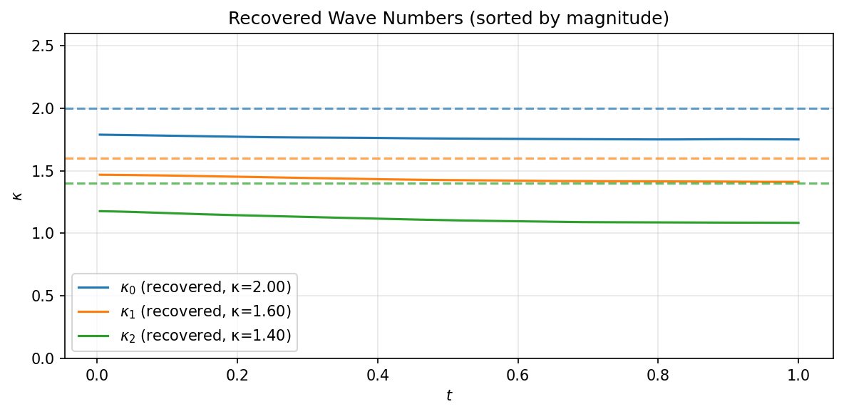 Figure 10: Recovered wave numbers for the 3-soliton configuration. The three eigenvalues are approximately recovered, though the accuracy degrades for the smaller-$\kappa$ modes. The slight negative slope in the recovered eigenvalues and the systematic offset illustrate the increased difficulty of the reconstruction as soliton number grows.
The spectral analysis confirms that the PINN preserves the isospectral property across all three modes, with the eigenvalue reconstruction remaining stable throughout the time domain. The accuracy is highest for the dominant modes (large $\kappa$) and degrades gradually for the weaker solitons, consistent with the finite-difference eigenvalue solver having more difficulty resolving shallow potential wells. The training also becomes more sensitive to the choice of initial positions and domain size as the number of solitons increases.
Discussion
The results here demonstrate that basic PINN formulations can be applied to the KdV equation in a fashion that preserves the underlying integrability, providing an example of how deep properties of exact solutions can be transferred to the learned model without additional inductive bias in the training. This is established by the local preservation of the KdV conservation hierarchy up to at least third order, and by verifying that the spectral properties (isospectrality and eigenfunction dynamics) are retained.
The study shows how pretraining is important for reducing the complexity of the optimization landscape by selecting the correct topological sector. At the same time, while accurate point estimates (small supervised residuals) can be obtained from the pretraining alone, such models fail almost immediately to constrain the derivatives, making them much less generalizable and flexible than the fully trained model.
In the case of the eigenvalues and eigenvectors, the pretrained model is able to capture these features well despite the failure to constrain the derivatives. In hindsight this is easy to understand since $L = -\partial_x^2 - u$ only depends (linearly) on $u$ and not on its derivatives. In many cases the full PINN training slightly degrades the eigenvalue reconstruction while substantially improving the derivative and conservation law residuals. PDE residual quality and spectral fidelity are complementary but distinct measures of solution quality.
In more challenging cases, the fully trained model exhibits a slight slope in the time dependence and a bias that affects all the eigenvalues. The pretrained model tends to work well until failing catastrophically by badly mixing modes, causing the eigenvalues to cross and discontinuous jumps to appear in the extracted eigenvectors. The full PINN model is more robust across a broader range of scattering data, but still exhibits a bias commensurate with the model’s inability to separate individual solitons. This is consistent with the behavior observed when comparing the accuracy of point-estimates of the pretrained and fully trained model and the derivative quantities.
Future Directions
A natural extension of this work is to introduce non-trivial reflection coefficients, which would admit broader classes of phenomena and provide an additional channel through which to test the spectral properties of the PINN. This requires a more sophisticated treatment of the Marchenko integral equation than is currently implemented. A related extension is to study solutions with periodic boundary conditions, where the relevant solutions are cnoidal waves.
Several directions emerge from the observations about training dynamics and spectral structure. The Darboux transformation, which strips off the dominant soliton to produce a lower-$N$ scattering problem, could be used to design an iterative training scheme that builds up the multi-soliton solution incrementally. The spectral analysis itself suggests a physics-informed basin-hopping strategy: if the eigenvalue extraction reveals that the model has settled in the wrong topological sector, the spectral data could be used to construct a correction that nudges the model toward the correct basin.
On the loss function side, the eigenvalue drift observed in some training runs suggests that a spectral regularizer penalizing departures from isospectrality could improve robustness without requiring knowledge of the exact eigenvalues. This would provide an integrability-preserving constraint that is independent of the PDE residual. Finally, the inverse scattering framework could be used to formulate inverse problems where the boundary data is incomplete but spectral constraints provide additional information to regularize the learned solution.
Appendix
$\tau$-Function Formulation
For numerical stability, the $N$-soliton solution is computed using the $\tau$-function formulation rather than direct evaluation of $\det M$. The $\tau$-function is defined as $\tau(x,t) = \det M$, and the potential is recovered via
\[u = 2\partial_x^2 \log \tau\]The determinant can be expanded over subsets $S \subseteq {1, \dots, N}$ as
\[\tau = \sum_{S \subseteq \{1,\dots,N\}} \prod_{\{i,j\} \subseteq S} \left(\frac{\kappa_i - \kappa_j}{\kappa_i + \kappa_j}\right)^2 \prod_{n \in S} \frac{c_n(t)^2}{2\kappa_n}\, e^{2\kappa_n x}\]This representation avoids computing the determinant of a potentially ill-conditioned matrix and allows the derivatives to be computed either analytically (by differentiating the known exponential dependence on $x$) or through autograd applied to the log-sum-exp form.