Weight Distributions in Transformer Attention Heads
Published:
Introduction
I’ve been interested in applying a physics framework to transformers involving dynamical systems and statistical mechanics. In this approach, the feature vectors representing tokens are interpreted as spins, the model weights play the role of interaction strengths between different token vectors, and the self-attention mechanism maps onto a thermodynamic average over these interactions. The structure of the model, with multiple attention heads, layers, and residual connections, allows for a large number of distinct, metastable equilibrium configurations: a spin glass system.
The object at the center of this picture is the bilinear form governing the attention logits for a single head,
\[\vec{Q}_{i}^{T} \cdot \vec{K_j} \,\,= \,\,\vec{x_i}^{T}W_{Q}^{T}W_{K}\vec{x_{j}} \,\,\equiv\,\, \vec{x_i}^{T}\, W_{QK}\, \vec{x_{j}}\]where $W_{QK} = W_{Q}^{T}W_{K}$ is the matrix that directly determines pairwise token interactions. In a physical system, this would be the coupling matrix specifying the energy of interaction between two spins. Understanding its statistical structure means understanding the geometry of the learned attention patterns.
At initialization, each attention head has the elements of $W_{Q}$ and $W_{K}$ drawn from some initial distribution, usually $\mathcal{N}(0,\sigma_0)$. The distribution for $W_{QK}$ is not set directly but rather follows from the distributions of the underlying weight matrices. Over the course of training the distribution changes shape to encode the information learned during back-propagation. This post examines the empirical distributions of these weight matrices across several transformer architectures and asks: how do the learned weight distributions differ from their initial Gaussian form, and what does this reveal about what models learn?
This is the first in a series of posts exploring transformer weights from a statistical physics perspective. Here I focus on establishing the basic distributional facts: the element-wise statistics of $W_Q$, $W_K$, and $W_{QK}$ for trained models, how these vary across layers and heads, and what distinguishes different model architectures. Subsequent posts will examine the singular value structure of $W_{QK}$ and the training dynamics revealed by the Pythia checkpoint suite.
The Low-Rank Structure of $W_{QK}$
In the typical transformer architecture, $W_{Q}$ and $W_{K}$ are $d_h \times d$ matrices, with $d_h = d / n_h$. Their product $W_{QK}$ is therefore a $d \times d$ matrix, but it has rank at most $d_h$. This low-rank constraint means that the smallest $d - d_h$ singular values are identically zero, and $W_{QK}$ operates only within a $d_h$-dimensional subspace of the full residual stream.
The effective rank of the matrix depends on the alignment of the singular vectors of $W_{Q}$ and $W_{K}$. These structures evolve dynamically during training and the actual rank of $W_{QK}$ for a trained model is emergent rather than fixed by the architecture. In a physics context, we try to associate the singular values of $W_{QK}$ with modes of definite energy, corresponding to particular directions in the spin space. The distribution of these modes encodes the effective degrees of freedom available to each attention head.
To develop some baseline intuition, I begin with a few numerical examples. The figures below show three-panel summaries of random matrices at $d$ = 1000: the element-wise probability density $P(W)$, the singular values ordered by index, and the spectral density $P(\lambda)$. All curves are averaged over multiple random draws.
The first figure shows full-rank random matrices with elements drawn from $\mathcal{N}(0,\sigma)$ for several values of $\sigma$. The element-wise distributions are, tautologically, Gaussian, and the singular values follow the Marchenko-Pastur distribution from random matrix theory.
![]()
Figure 1: Full-rank random matrices at $d$ = 1000 for several values of $\sigma$. Left: element-wise density $P(W)$. Center: singular values vs. index. Right: spectral density $P(\lambda)$.
The next figure introduces the low-rank structure relevant to $W_{QK}$. Setting $W_{QK} = W_{Q}^{T}W_{K}$ with $d_h = d/2$ = 500, the element-wise distribution narrows and the singular value spectrum develops a sharp transition at the $d_h$-th index, dropping effectively to zero. The spectral density develops a gapped structure with support over two disconnected domains.
![]()
Figure 2: Low-rank random matrix products $W_{QK} = W_Q^T W_K$ at $d$ = 1000 and $d_h$ = 500, for several values of $\sigma$. The singular value spectrum exhibits a sharp cutoff at $d_h$, and the spectral density develops a gap.
Varying $d_h$ while keeping $\sigma$ = 1 reveals the expected behavior: as the rank decreases (more heads), the gap widens and the element-wise distribution narrows. The element-wise standard deviation scales as $\sigma_{W_{QK}} \propto \sqrt{d_h / d} = 1/\sqrt{n_h}$, and the entropy follows $S = \frac{1}{2}\ln(2\pi e / n_h)$. The spectral edge positions are given approximately by the Marchenko-Pastur bounds: $\lambda_{\pm} = \sqrt{d_h}(1 \pm \sqrt{d / d_h})$.
![]()
Figure 3: Effect of varying $d_h$ at fixed $d$ = 1000 and $\sigma$ = 1. Left: element-wise distributions narrow as $1/\sqrt{n_h}$. Center: singular values with cutoff at $d_h$. Right: spectral density transitions from gapped (low rank) to continuous (full rank).
These baselines establish what we should expect from the spectral structure of random, untrained weight matrices.
Entropy and KL Divergence of Random $W_{QK}$
The element-wise distribution of $W_{QK} = W_Q^T W_K$ is not Gaussian by construction: each element is a sum of $d_h$ products of Gaussian random variables. However, at the matrix sizes relevant to transformer architectures, the central limit theorem drives the element-wise distribution very close to Gaussian. This can be verified empirically without deriving the exact distribution.
Figure 4 shows the standard deviation and differential entropy of random $W_{QK}$ matrices as a function of $d_h$ at fixed $d$ = 1000 with $\sigma$ = 1. The left panel confirms that $\sigma_{W_{QK}} = \sqrt{d_h/d}$ and that the entropy follows $S = \frac{1}{2}\ln(2\pi e\, d_h/d)$, which is just the Gaussian entropy evaluated at that $\sigma$. The right panel shows the KL divergence $D_{\text{KL}}(P_{W_{QK}} | \mathcal{N}(0,\sigma))$, where $\sigma$ is the measured standard deviation of the same matrix. This quantity is identically zero for a Gaussian and measures the total departure from normality. Across the full range of $d_h$, the KL divergence is at most $\sim 10^{-3}$ and falls toward zero as $d_h$ increases, confirming that the element-wise distribution converges to Gaussian as expected from the central limit theorem. The KL is largest at small $d_h$ where each element is a sum of fewer Gaussian products and the CLT has not fully converged, and negligible by $d_h \gtrsim 200$.
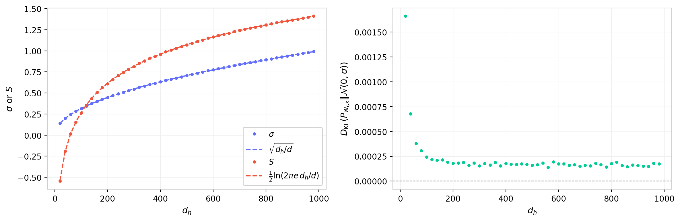
Figure 4: Properties of random $W_{QK}$ matrices vs. head dimension $d_h$ at $d$ = 1000. Left: standard deviation and entropy, with analytic Gaussian predictions (dashed). Right: $D_{\text{KL}}(P_{W_{QK}} \| \mathcal{N}(0,\sigma))$. The KL divergence falls toward zero as $d_h$ increases, reflecting CLT convergence to Gaussian; the residual non-Gaussianity at small $d_h$ reflects the finite number of terms in each element's sum.
This result has a practical consequence: when comparing trained weight distributions to a Gaussian baseline, we do not need to account for the low-rank product structure of $W_{QK}$. The Gaussian with the same $\sigma$ is the correct reference for both $W_Q$ and $W_{QK}$, and any departure from it in trained models can be attributed to learning rather than to the matrix product structure. Note also that $\Delta S = -D_{\text{KL}}(P | \mathcal{N}(0,\sigma))$ when the distribution has zero mean and variance $\sigma^2$, so the entropy residual and KL divergence are the same quantity up to a sign.
A notebook (low_rank_SVD_systematics.ipynb) is available with further exploration of these baselines.
Models and Data
The analysis uses pre-trained models available on HuggingFace. For each model, I extract the $W_Q$, $W_K$, and $W_{QK}$ matrices for every attention head across all layers, then compute element-wise histograms, summary statistics (mean, standard deviation, skewness, kurtosis), entropy measures, and the full singular value decomposition.
| Model | $d$ | $n_h$ | $d_h$ | Layers | Parameters | Notes |
|---|---|---|---|---|---|---|
| GPT-2 (small) | 768 | 12 | 64 | 12 | 124M | Primary illustration model |
| GPT-2 (medium) | 1024 | 16 | 64 | 24 | 355M | |
| GPT-2 (large) | 1280 | 20 | 64 | 36 | 774M | |
| GPT-2 (XL) | 1600 | 25 | 64 | 48 | 1.5B | |
| LLaMA 3.1 8B | 4096 | 32 | 128 | 32 | 8B | Grouped-query attention |
| Mistral 7B v0.3 | 4096 | 32 | 128 | 32 | 7B | Grouped-query attention |
| Pythia-70M | 512 | 8 | 64 | 6 | 70M | |
| Pythia-160M | 768 | 12 | 64 | 12 | 160M | |
| Pythia-410M | 1024 | 16 | 64 | 24 | 410M | |
| Pythia-1B | 2048 | 8 | 256 | 16 | 1B | |
| Pythia-1.4B | 2048 | 16 | 128 | 24 | 1.4B | |
| Pythia-2.8B | 2560 | 32 | 80 | 32 | 2.8B | |
| Pythia-6.9B | 4096 | 32 | 128 | 32 | 6.9B | |
| Pythia-12B | 5120 | 40 | 128 | 36 | 12B |
Table 1: Models included in this study. All models are publicly available on HuggingFace. LLaMA and Mistral use grouped-query attention (GQA), where the number of K/V heads is smaller than Q heads; K heads are expanded via repeat_interleave to match the Q head count before computing $W_{QK}$. Pre-computed statistics for all models are available at angerami/weight_study_ana-004.
The Pythia model suite, developed by EleutherAI, provides an additional dimension: 154 training checkpoints from initialization to convergence, enabling the study of how these distributions evolve during training. The time-evolution analysis is deferred to a subsequent post, but the Pythia models appear in the cross-model comparisons below.
All pre-computed statistics are published on HuggingFace under angerami/weight_study_ana-004 (cross-model, all 14 models) and angerami/pythia-{size}-deduped_weight_evolution_001 (training dynamics, deferred to a later post). An interactive Streamlit dashboard for exploring the data is available on HuggingFace Spaces.
Results: Weight Distributions in GPT-2
Per-Head Distributions
To establish some expectations we start with GPT-2 (small), which has $d$ = 768, 12 layers, and 12 attention heads per layer. The $W_Q$ and $W_K$ matrices each contain 768 $\times$ 768 / 12 $\approx$ 49,000 elements per head, providing a substantial statistical sample.
The figure below shows histograms of the $W_Q$ weight distribution for the 12 attention heads in layer 0. Each of these can be thought of as a separate system of $\sim$ 49,000 degrees of freedom. At initialization all heads are drawn from the same distribution $\mathcal{N}(0, \sigma_0)$, but as you can see they evolve differently during training.
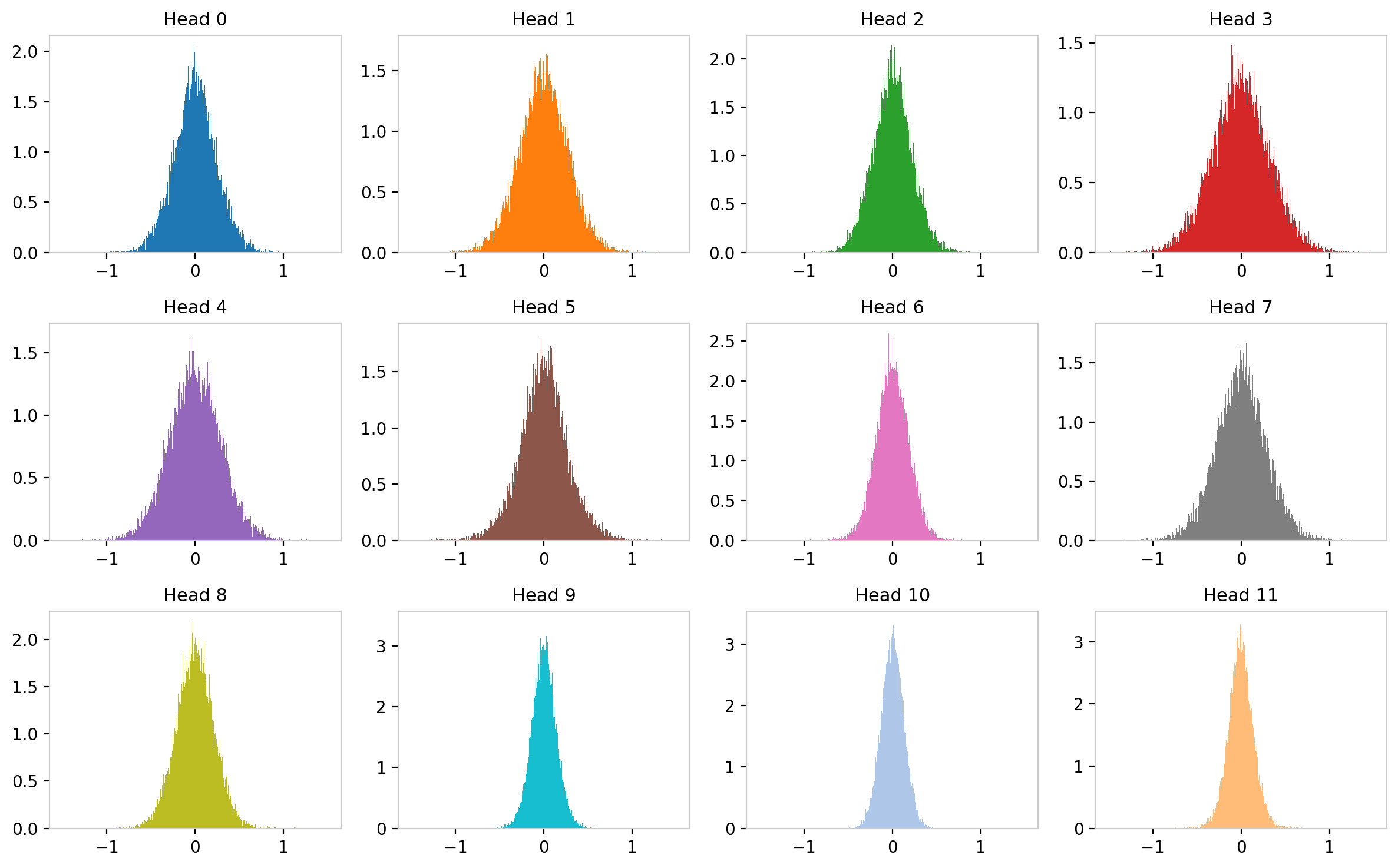
Figure 5: $W_Q$ weight distributions for 12 attention heads in GPT-2 layer 0 (linear scale). Despite identical initialization, the trained distributions develop distinct widths and shapes.
The same distributions on a logarithmic vertical scale, with Gaussian fits overlaid, reveal not only that the distributions have different $\sigma$ values but that they show different levels of deviation from normality. Some heads remain well-described by a Gaussian; others develop heavier tails, particularly on the negative side.
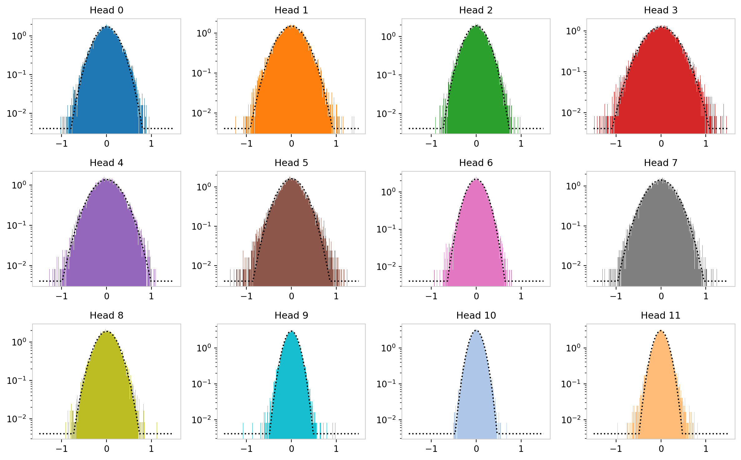
Figure 6: Same distributions as Figure 5, on logarithmic scale with Gaussian fits. Deviations from the Gaussian envelope, visible as excess probability in the tails, vary substantially across heads.
Distributions Across the Full Model
To summarize the entire model, the figure below shows the $W_Q$ distributions for all heads across all layers as a 2D heatmap, where each row corresponds to one attention head (grouped by layer) and the color indicates log probability density. The distributions generally narrow as one goes deeper in the network. While different heads in the same layer tend to be similar, the figure reveals a few cases where particular heads show very different behavior from these general trends.
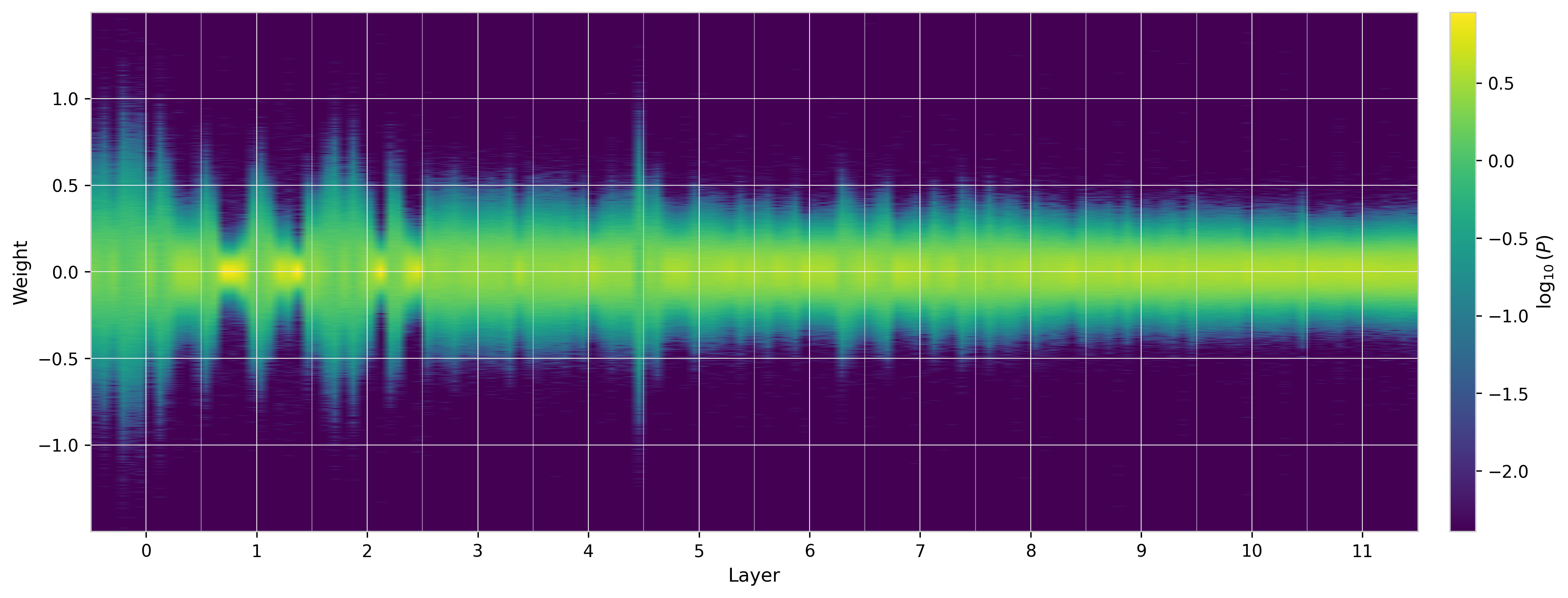
Figure 7: $W_Q$ weight distributions across all heads and layers of GPT-2 (small), shown as a 2D heatmap on logarithmic color scale. Each row is one head; layers are separated by dashed lines. The general trend is narrowing with depth, but individual heads can deviate substantially.
Summary Statistics
Two summary statistics, the standard deviation $\sigma$ and the differential entropy $S = -\int P(w) \ln P(w)\, dw$ (estimated via KDE), confirm the behavior observed above. The distributions qualitatively narrow with depth, but there are large variations among heads within the same layer that are of a similar scale as the overall downward trend.
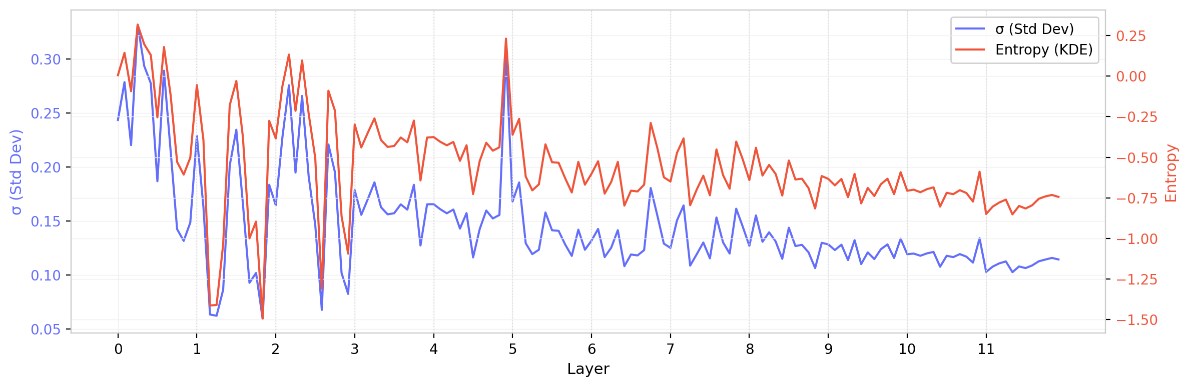
Figure 8: $W_Q$ standard deviation (blue) and entropy (red) across all attention heads in GPT-2 (small), ordered by layer. Vertical dashed lines separate layers. Both statistics show a general decrease with depth, modulated by substantial head-to-head variation within each layer.
GPT-2 XL
The same analysis for GPT-2 XL ($d$ = 1600, 25 heads, 48 layers) provides a useful comparison. The 2$\times$ increase in model dimension results in a 4$\times$ increase in the number of matrix elements per head, which should reduce sampling fluctuations on statistical estimators by roughly 2$\times$. The summary statistics plot does indeed look smoother. However, while this model exhibits some of the same trends as GPT-2 (small), there is a notable resurgence in the later layers: the standard deviation and entropy, after decreasing through the middle layers, increase again toward the output.
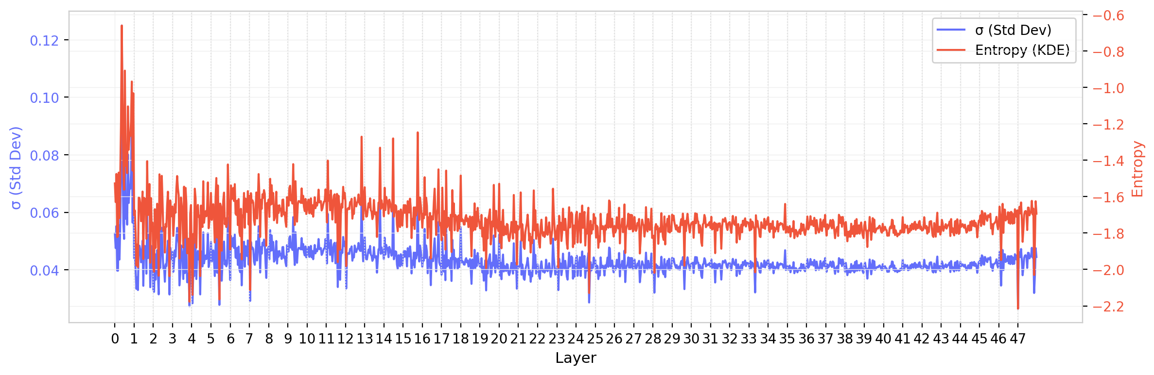
Figure 9: $W_Q$ standard deviation and entropy for GPT-2 XL. Unlike GPT-2 (small), both statistics show a non-monotonic pattern with a resurgence in later layers.
Results: $W_{QK}$ Distributions
Amplification of Non-Gaussianity
The element-wise distributions of $W_Q$ and $W_K$ individually remain approximately Gaussian across most heads and layers. Their product $W_{QK}$, however, tells a different story. Small deviations from normality in the individual matrices are dramatically amplified by the matrix product. The $W_{QK}$ distributions develop heavy tails that grow much faster than those in the individual matrices. For these distributions (e.g. head 8), the Gaussian fit matches well in the core, but undershoots the data in the tails. In other cases (e.g. head 1) the distribution falls too steeply near its maximum, resulting in something that is too pointy to be compatible with a Gaussian.
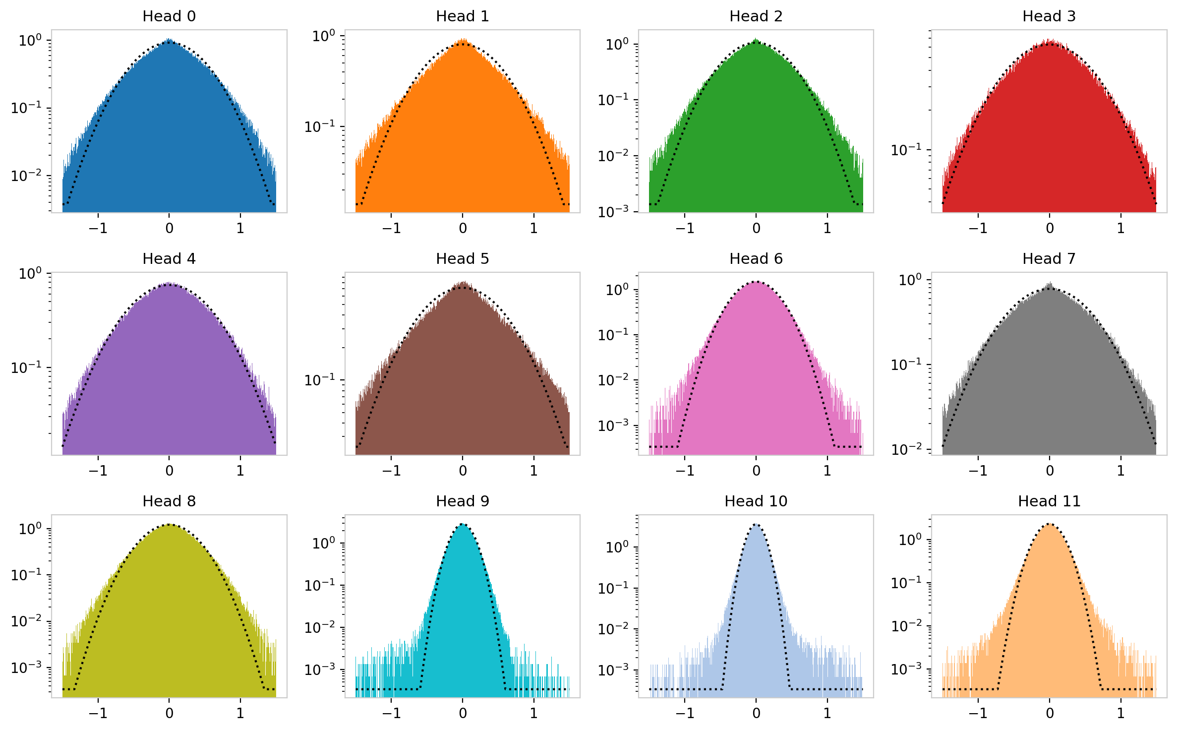
Figure 10: $W_{QK}$ weight distributions for GPT-2 layer 0 on logarithmic scale. Compared to the individual $W_Q$ distributions (Figure 6), the deviations from Gaussianity are substantially larger, with pronounced asymmetric tails.
This asymmetry is physically interesting. The $W_{QK}$ matrix is the pre-softmax attention logit matrix, so its statistical structure directly encodes what the model has learned about which tokens should attend to which. A heavier negative tail means more extreme “don’t attend” signals than “do attend” signals. In the language of the softmax function, strong negative logits are effectively suppressed to zero attention weight, so the model appears to learn structured inhibition patterns.
$W_{QK}$ Across the Full Model
The 2D heatmap for $W_{QK}$ shows more dramatic structure than the individual weight matrices. The variation across layers and heads is more pronounced, and the tails (visible as extended color in the heatmap wings) are clearly wider than what a Gaussian with the same $\sigma$ would produce.
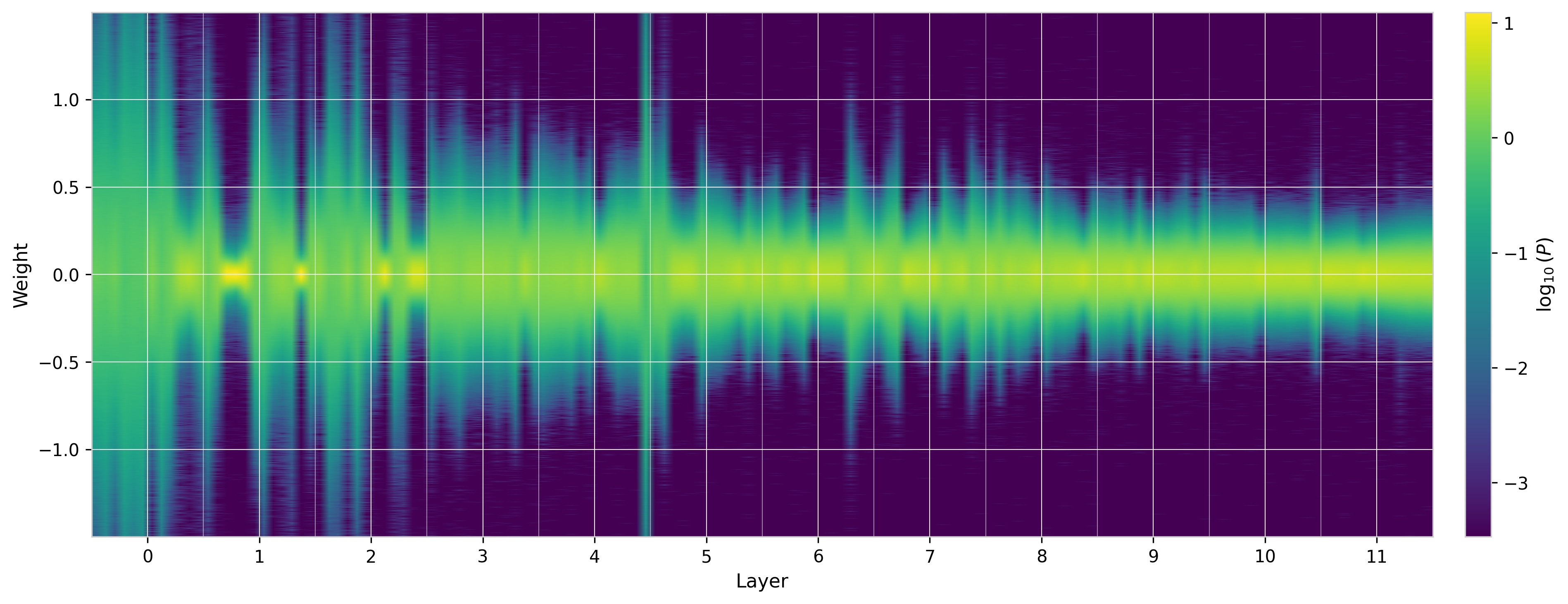
Figure 11: $W_{QK}$ distributions across all heads and layers of GPT-2 (small). The non-Gaussian character is visible as extended tails (color at large $|w|$) beyond what the central peak width would predict.
Cross-Model Comparison
Comparing across model families reveals both universal features and notable differences. The general pattern, where $W_Q$ and $W_K$ remain approximately Gaussian while $W_{QK}$ develops heavier tails, is consistent across all architectures studied. However, the scale and shape of the distributions vary substantially.
The Mistral–LLaMA Sigma Anomaly
Despite identical architecture parameters ($d$ = 4096, 32 heads, 32 layers), Mistral’s $W_Q$ and $W_K$ standard deviations are 5–10$\times$ smaller than LLaMA’s, and this difference compounds in $W_{QK}$.
One hypothesis is that the two models use different normalization factors in the attention scaling. If one model uses $1/\sqrt{d}$ while the other uses $1/\sqrt{d_h}$, the ratio of effective scales is $\sqrt{d/d_h} = \sqrt{4096/128} \approx$ 5.66, which matches the observed ratio nearly exactly. This finding illustrates that models with identical parameter counts and architecture can exhibit fundamentally different weight characteristics after training, suggesting different optimization landscapes.
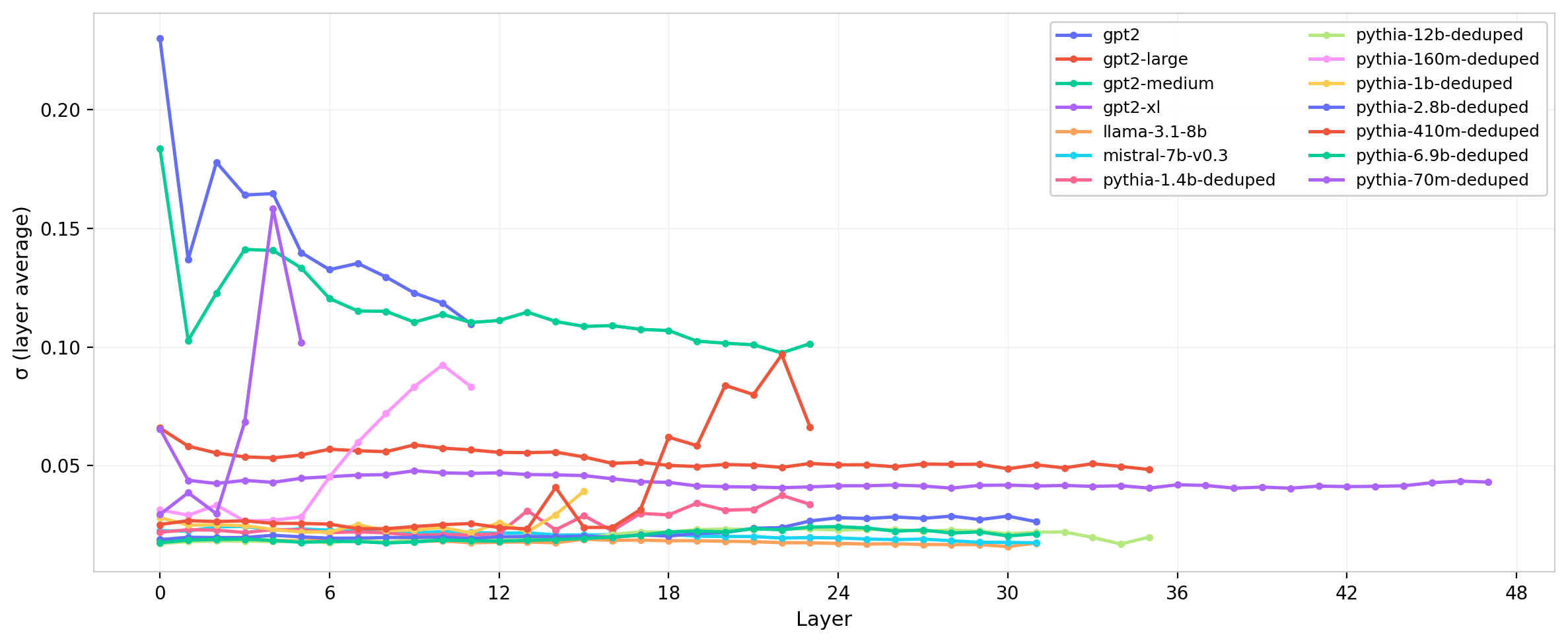
Figure 12: Standard deviation of $W_Q$ across layers for all model families. The Mistral–LLaMA scale difference is clearly visible despite identical architectural dimensions.
The same comparison for $W_{QK}$ is shown in Figure 13. The scale separation between Mistral and LLaMA is amplified in the product matrix, consistent with the $\sigma_{W_{QK}} \propto \sigma^2$ scaling expected from the random matrix baseline.
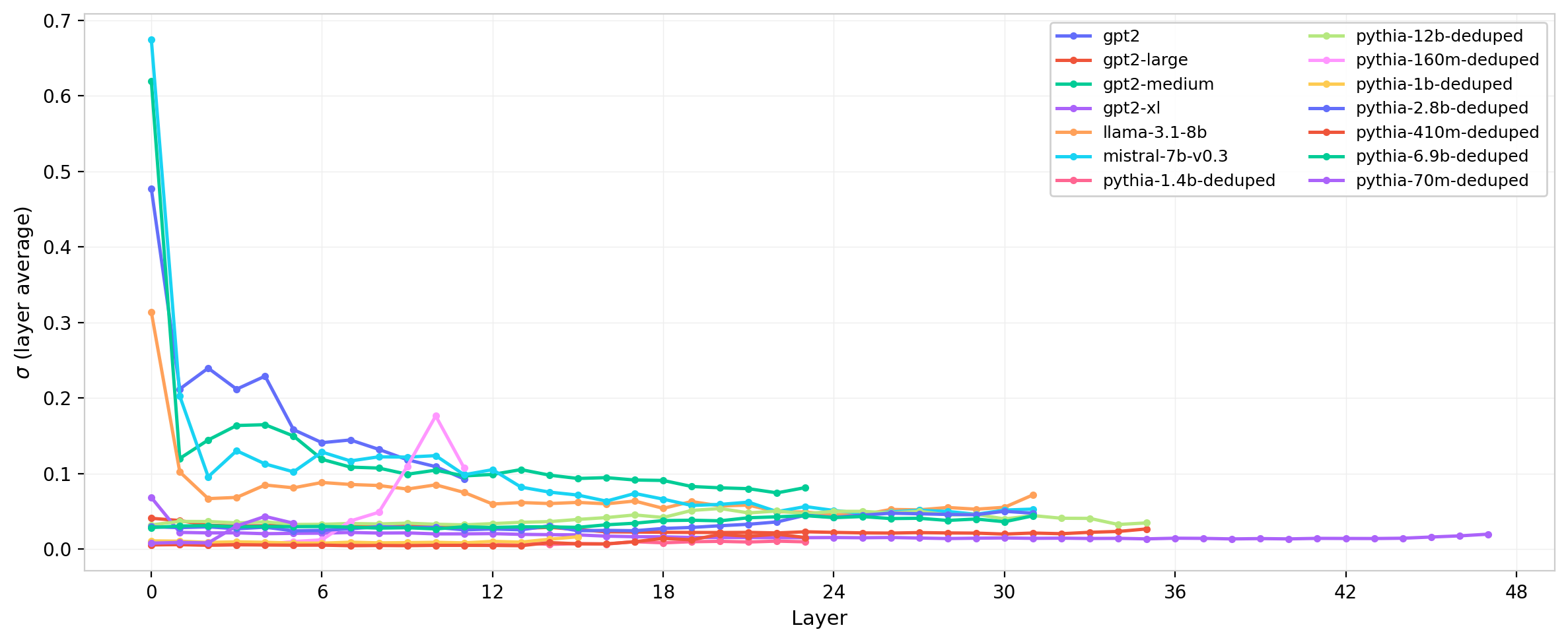
Figure 13: Standard deviation of $W_{QK}$ across layers for all model families. The Mistral–LLaMA scale separation is amplified relative to the individual weight matrices (Figure 12), reflecting the quadratic $\sigma$ scaling of the matrix product.
The cross-model comparisons in this post are primarily qualitative; a quantitative comparison against Monte Carlo-simulated Gaussian expectations is deferred to future work.
Entropy and the Gaussian Reference
The differential entropy $S = -\int P(w) \ln P(w)\, dw$ and the standard deviation $\sigma$ are not independent: for a Gaussian distribution, $S = \frac{1}{2}\ln(2\pi e\,\sigma^2)$. This provides a useful reference curve. Distributions that match the Gaussian prediction have entropy fully determined by their width; deviations indicate structure in the shape of the distribution beyond what $\sigma$ alone captures.
Figure 14 plots the measured entropy against $\sigma$ for every attention head in every model, with the Gaussian prediction shown as a solid curve. For $W_Q$ (left panel), the data points cluster tightly along the analytic curve, consistent with the observation that individual weight matrices remain approximately Gaussian after training. The right panel shows the same comparison for $W_{QK}$. Here the numerical reference curve for random $W_{QK}$ matrices at GPT-2 dimensions ($d$ = 768, $d_h$ = 64) is shown as a dashed red line; it falls directly on top of the Gaussian prediction, confirming that at these matrix sizes the central limit theorem has fully converged and the product-of-Gaussians distribution is effectively indistinguishable from a Gaussian in its entropy. This result holds across all model sizes in the study, establishing the Gaussian as a universal reference for both $W_Q$ and $W_{QK}$.
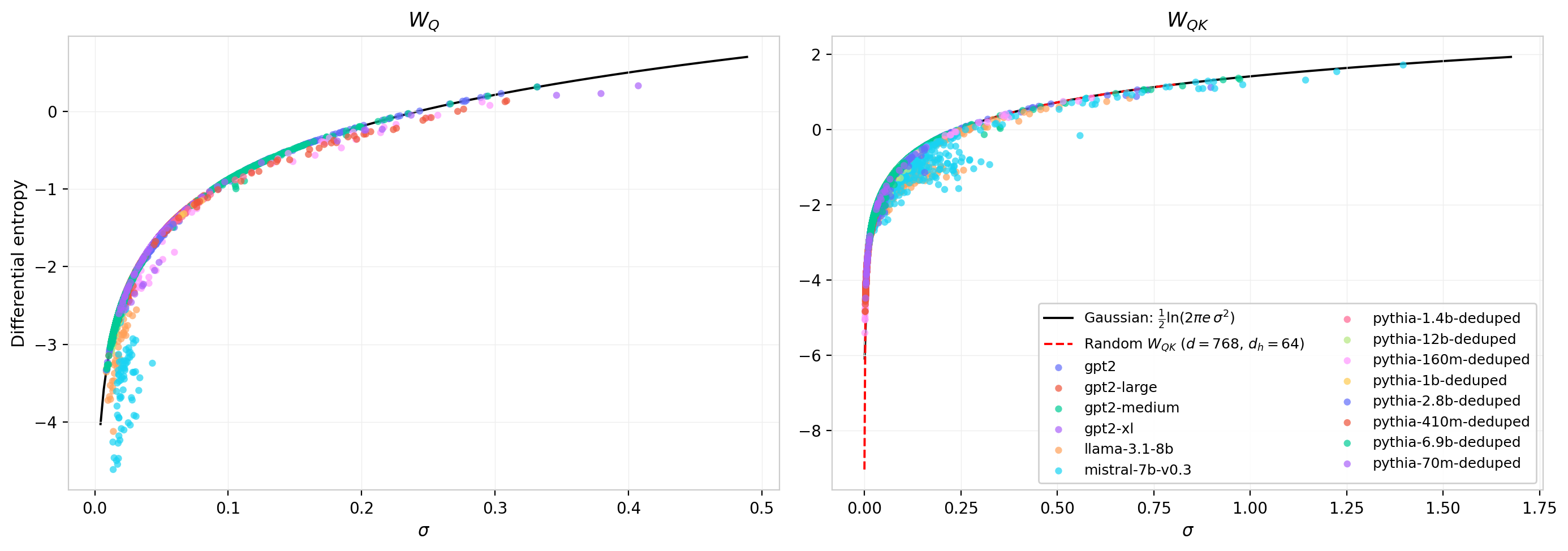
Figure 14: Differential entropy vs. standard deviation for all attention heads across all models. Left: $W_Q$. Right: $W_{QK}$. The solid black curve is the Gaussian prediction $S = \frac{1}{2}\ln(2\pi e\,\sigma^2)$; the dashed red curve (right panel) is the numerical result for random $W_{QK}$ at $d$ = 768, $d_h$ = 64. Both references coincide, confirming the Gaussian as the appropriate baseline.
To isolate the deviations, Figure 15 subtracts the Gaussian prediction and plots the residual $\Delta S = S_{\text{measured}} - \frac{1}{2}\ln(2\pi e\,\sigma^2)$. For a perfect Gaussian, $\Delta S = 0$. A negative residual indicates a distribution with less entropy than a Gaussian of the same width, pointing to sharper peaks or more concentrated probability mass; a positive residual would indicate heavier tails or broader structure.
For $W_Q$ (left panel), the residuals are small and predominantly negative, consistent with slight sub-Gaussian character: the trained distributions are marginally more concentrated than their Gaussian envelopes. For $W_{QK}$ (right panel), the residuals are systematically more negative, reflecting the heavier-tailed, non-Gaussian character observed in the per-head distributions above. Despite the heavy tails visible on logarithmic scale, the net effect on the entropy is a reduction relative to the Gaussian prediction. This is consistent with a distribution that concentrates more probability near its center while simultaneously extending farther into the tails than a Gaussian would: the tail weight is too sparse to compensate for the central concentration.
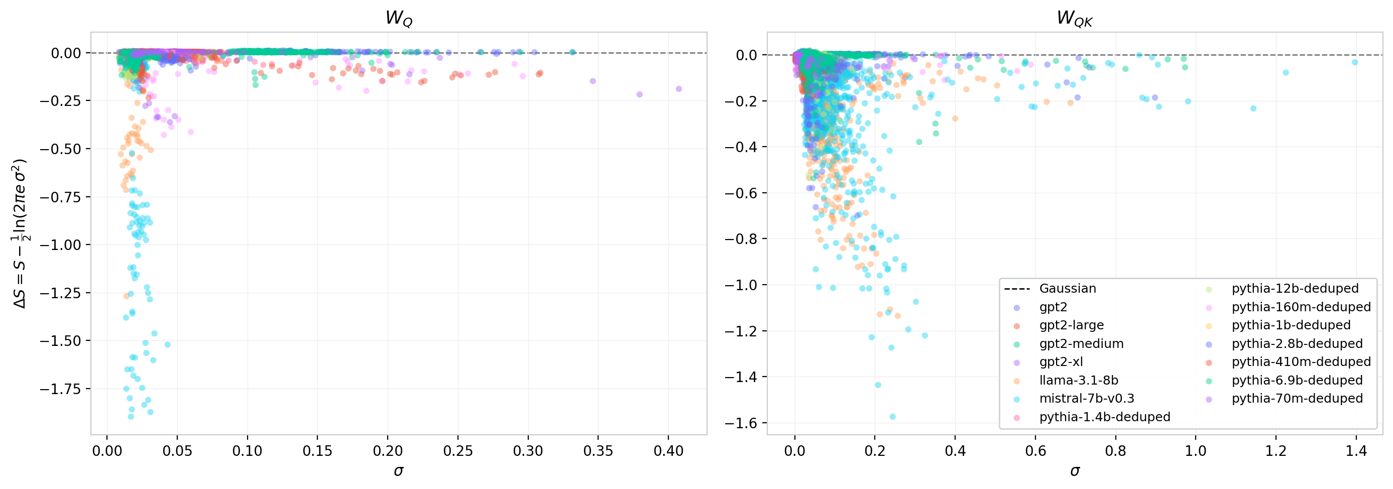
Figure 15: Entropy residual $\Delta S = S - \frac{1}{2}\ln(2\pi e\,\sigma^2)$ vs. $\sigma$ for all heads and models. Left: $W_Q$. Right: $W_{QK}$. Negative values indicate sub-Gaussian entropy. The $W_{QK}$ residuals are systematically larger in magnitude, reflecting the amplified non-Gaussianity of the matrix product.
Gaussian Fit Quality
As a complement to the entropy measures, one can quantify non-Gaussianity by directly fitting a Gaussian to each per-head distribution and measuring how well the fitted parameters reproduce the empirical ones. The fitted standard deviation $\sigma_{\mathrm{fit}}$ (obtained by maximum-likelihood fitting) and the KL divergence between the empirical distribution and the fitted Gaussian provide two independent diagnostics.
Figures 16 and 17 show these quantities layer by layer for GPT-2 (small), for $W_Q$ and $W_{QK}$ respectively. The fitted $\sigma_{\mathrm{fit}}$ tracks the empirical $\sigma$ closely but is systematically slightly smaller, consistent with the sub-Gaussian character noted above: the Gaussian fit places less weight in the tails and correspondingly tightens the inferred width. The KL divergence is largest in the early layers, where $\sigma$ is largest and the distributions develop the most pronounced non-Gaussian structure, and decreases toward the later layers.
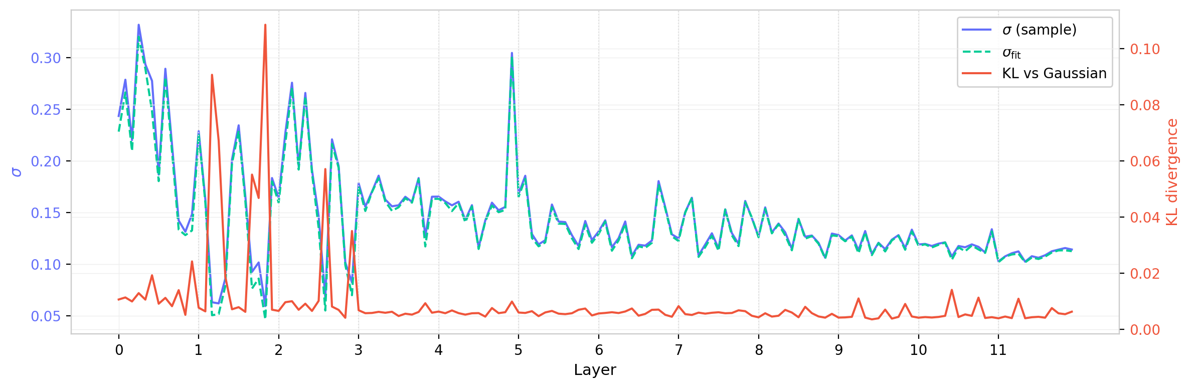
Figure 16: $W_Q$ fitted standard deviation $\sigma_{\mathrm{fit}}$ (green dashed) and empirical $\sigma$ (blue), together with KL divergence vs. Gaussian (red, right axis), across all layers and heads of GPT-2 (small). The KL divergence is largest in early layers where the distributions are widest.
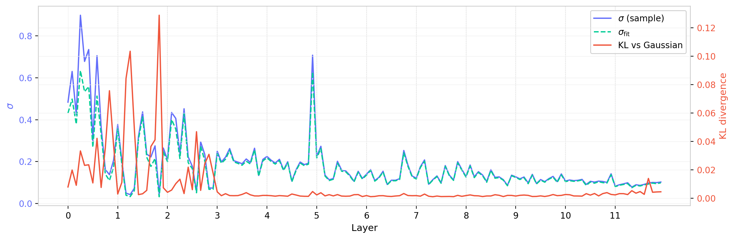
Figure 17: Same as Figure 16 for $W_{QK}$. The KL divergence is substantially larger than for $W_Q$, with pronounced peaks in the first few layers, reflecting the amplified non-Gaussianity of the matrix product.
Figures 18 and 19 extend this comparison across all models. Figure 18 shows $\sigma_{\mathrm{fit}}$ against $\sigma$ for every head in the dataset (top row) and the residual $\sigma_{\mathrm{fit}}^2 - \sigma^2$ (bottom row). For $W_Q$ the relationship is nearly linear with a slight negative offset; for $W_{QK}$ the scatter is larger and the residuals grow with $\sigma$, indicating increasing deviation from Gaussian as the matrix product amplifies structure. Figure 19 shows the KL divergence against $\sigma$ directly: the non-Gaussianity of $W_Q$ concentrates at intermediate $\sigma$ values with a broad scatter, while for $W_{QK}$ the KL values extend to higher magnitudes and show greater model-to-model variability.
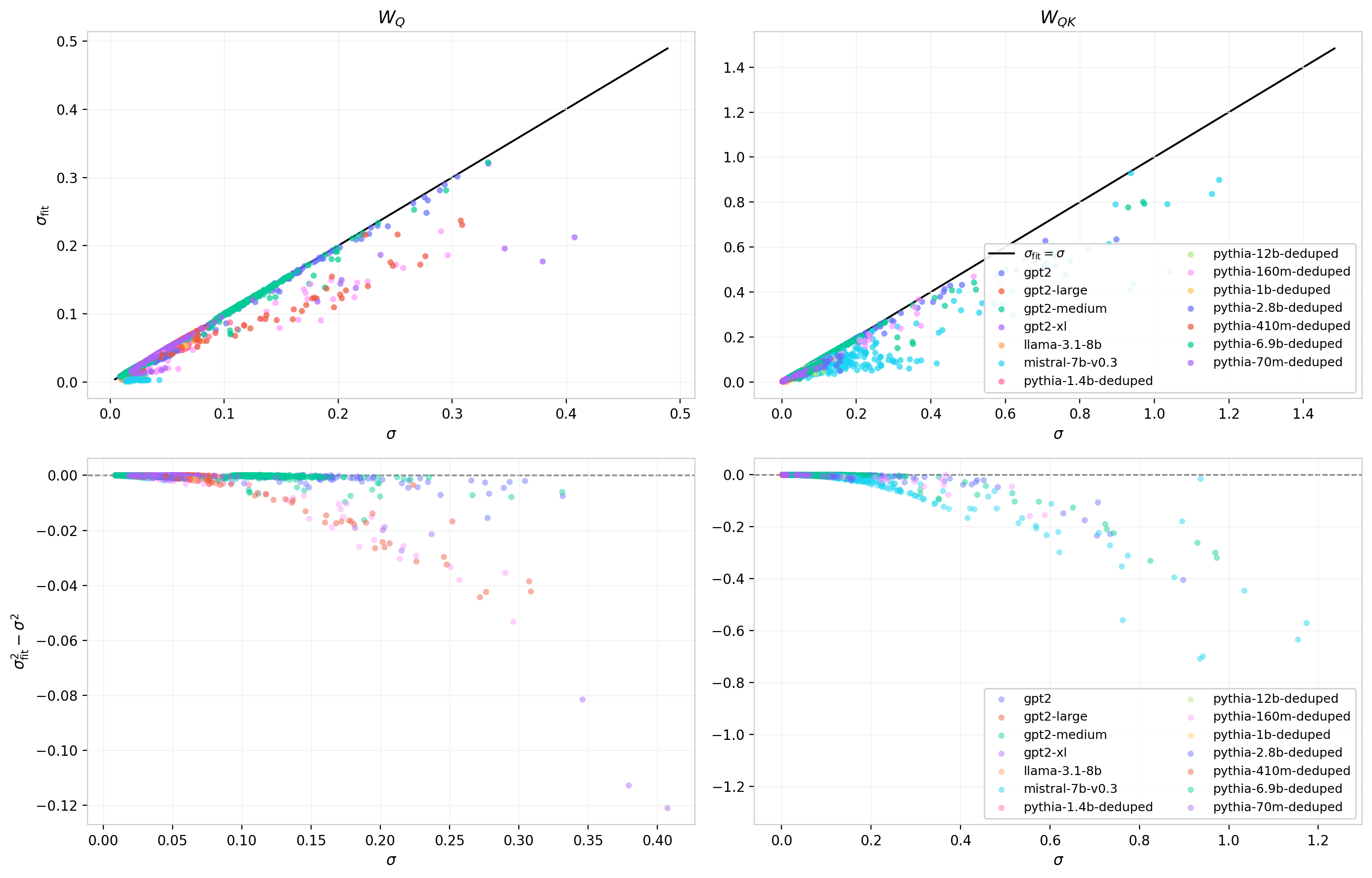
Figure 18: Fitted vs. empirical standard deviation across all heads and models. Top: $\sigma_{\mathrm{fit}}$ vs. $\sigma$ with identity reference. Bottom: residual $\sigma_{\mathrm{fit}}^2 - \sigma^2$. Left: $W_Q$. Right: $W_{QK}$. The systematic negative residual reflects sub-Gaussian character in the trained distributions.
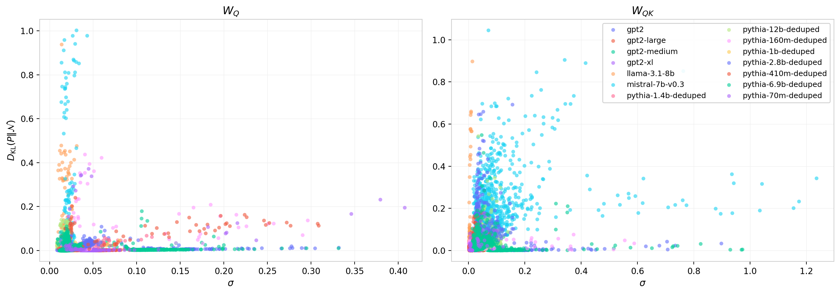
Figure 19: KL divergence $D_{\mathrm{KL}}(P \| \mathcal{N}(0,\sigma))$ vs. empirical $\sigma$ for all heads and models. Left: $W_Q$. Right: $W_{QK}$. The non-Gaussianity of $W_{QK}$ is systematically larger and extends across a wider range of $\sigma$ values, consistent with the amplification seen in the entropy residuals.
Correlations Among Per-Head Statistics
In models without bias, such as LLaMA and Mistral, the mean remains numerically small but is free to develop some information about the scale. For these models it is straightforward to see how a small non-Gaussian mixture develops in some heads by studying correlations among the moments.
The mean, standard deviation, skewness, and kurtosis and their correlations are shown in the corner plot below for LLaMA and Mistral.
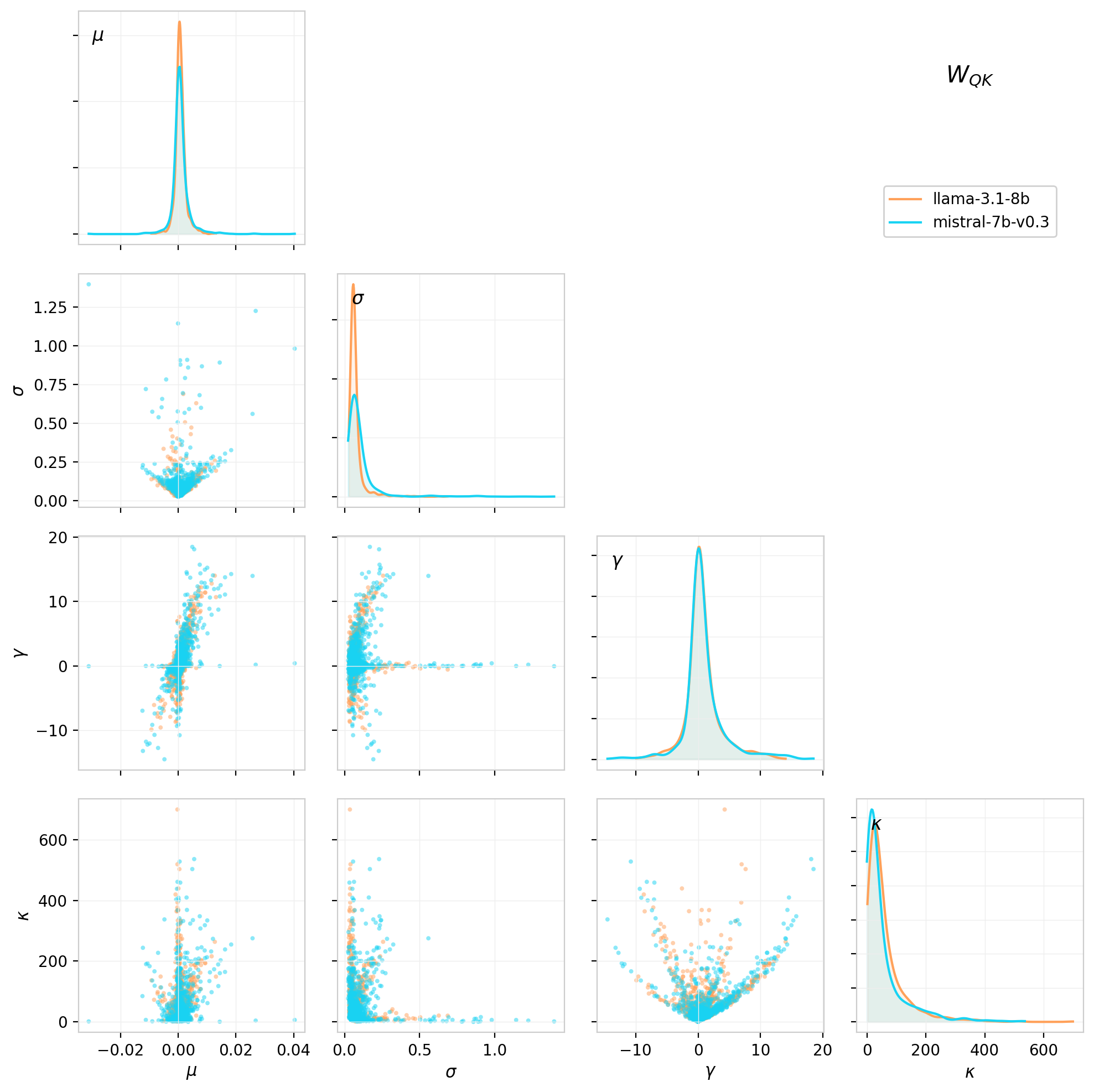
Figure 20: Corner plot for the first four moments of the $W_{QK}$ weight distributions for each attention head, shown for LLaMA 3.1 8B (orange) and Mistral 7B v0.3 (blue). The band structures in the 2D correlations suggest many heads whose distributions are well-described by a Gaussian with a small mixture component.
In the case of a mixture distribution with $N(0,\sigma_0)$ with weight $p$ and an additional localized component at $a$ with weight $1-p$, the moments are approximately related as follows:
\[\mu \approx p·a \,,\quad \sigma^2 ≈ (1-p)\sigma_{0}² + p·a^2 \,,\quad \gamma \propto p·a^3 / \sigma^3 \,,\quad \kappa ∝ p·a^4 / \sigma^4\]Different heads end up with different $p$ values, which trace out fixed curves in the moment correlation space rather than filling it. The easiest case to see is in the $\gamma - \kappa$ correlation, which is limited by the inequality (Pearson’s Bound): \(\kappa \geq \gamma^2 + 1\,,\) when this limit is saturated it gives rise to parabolic curve in the correlation,
It is also evident in the $\mu - \sigma$ correlation, where the $\sigma$ values are limited from below approximately as:
\[\sigma(\mu) \gtrsim \frac{1}{\sqrt{p}}\sqrt{\mu^2 + \frac{1-p}{p}\sigma_0^2 }\,,\]and in the $\gamma - \sigma$ correlation:
\[\sigma(\gamma) \gtrsim \sqrt{\frac{1-p}{p}} \frac{\sigma_0}{\sqrt{1 - (p\gamma)^{2/3}}}\]Values clustering at or near the edge of this limit are characteristic of weight distributions that are close to a two-point or low-entropy mixture. In cases where this simple mixture picture begins to fall apart the correlations fill in the bulk of the distribution.
In models with bias, the moments are more complicated to interpret since information is distributed between the weight and bias contributions. In these cases the mean primarily serves as a nuisance parameter. The loss of scale effectively collapses the dynamic range to be able to see this behavior.
What Comes Next
This post establishes the basic distributional facts: individual weight matrices $W_Q$ and $W_K$ remain well-behaved and approximately Gaussian, but their product $W_{QK}$ develops structured non-Gaussianity with heavy, asymmetric tails. These deviations from the random-matrix baselines are the signal of learned structure.
The next post in this series examines the singular value decomposition of $W_{QK}$, which moves beyond the element-wise marginal statistics explored here to characterize the spectral structure: how many effective dimensions each head uses, how the spectrum differs from the Marchenko-Pastur predictions, and what this reveals about the geometry of learned attention patterns. The third post will use the Pythia training checkpoints to study how all of these structures emerge during training.
The code, data, and interactive dashboards for reproducing and extending this analysis are available at the links above.